Buy low sell high on big tech stocks?

tidyTuesday

Author

Chun Su

Published

February 18, 2023

I am interested in Big Tech Stock Prices since I personally hold several big Tech stocks and experienced bloody plummeting in the last year. As an amateur investor, I have been always questioning my investing strategies, and wondering how different strategies result in the gains. Retrospect analysis is a good way to answer the question partially.

In this TidyTuesday¹ exercise, I will use strategy of “buy low sell high” at 52 weeks cycle on these big tech stocks, and see which company fits this strategy the best.

Code

library(tidyverse)
library(lubridate)
theme_set(theme_bw())

Code

big_tech_stock_prices <- readr::read_csv('https://raw.githubusercontent.com/rfordatascience/tidytuesday/master/data/2023/2023-02-07/big_tech_stock_prices.csv')
big_tech_companies <- readr::read_csv('https://raw.githubusercontent.com/rfordatascience/tidytuesday/master/data/2023/2023-02-07/big_tech_companies.csv')

Example of “buy low sell high” strategy in APPL

To compose functions, I will use Apple stock (APPL) as an example. Starting from the earliest available date, observe for one period (52 weeks), then start to invest afterwards.

Code

stock_symbol <- 'AAPL'

period <- 52*7

# first date ready to invest
start_date <- big_tech_stock_prices |> 
    filter(stock_symbol==!!stock_symbol) |> 
    slice(which.min(date)) |> 
    mutate(date = as.character(date + period)) |> 
    pull(date) |> 
    as.Date() # "2011-01-03"

# data.frame ready to invest
df <- big_tech_stock_prices |> 
    filter(stock_symbol==!!stock_symbol, date >= start_date)

Code

# plot whole time price trends
big_tech_stock_prices |> 
    filter(stock_symbol==!!stock_symbol) |> 
    ggplot(aes(x = date, y = low)) +
    geom_line() +
    geom_vline(aes(xintercept = start_date), color = "red") +
    ggtitle(glue::glue("{stock_symbol} stock price trend since 2010"))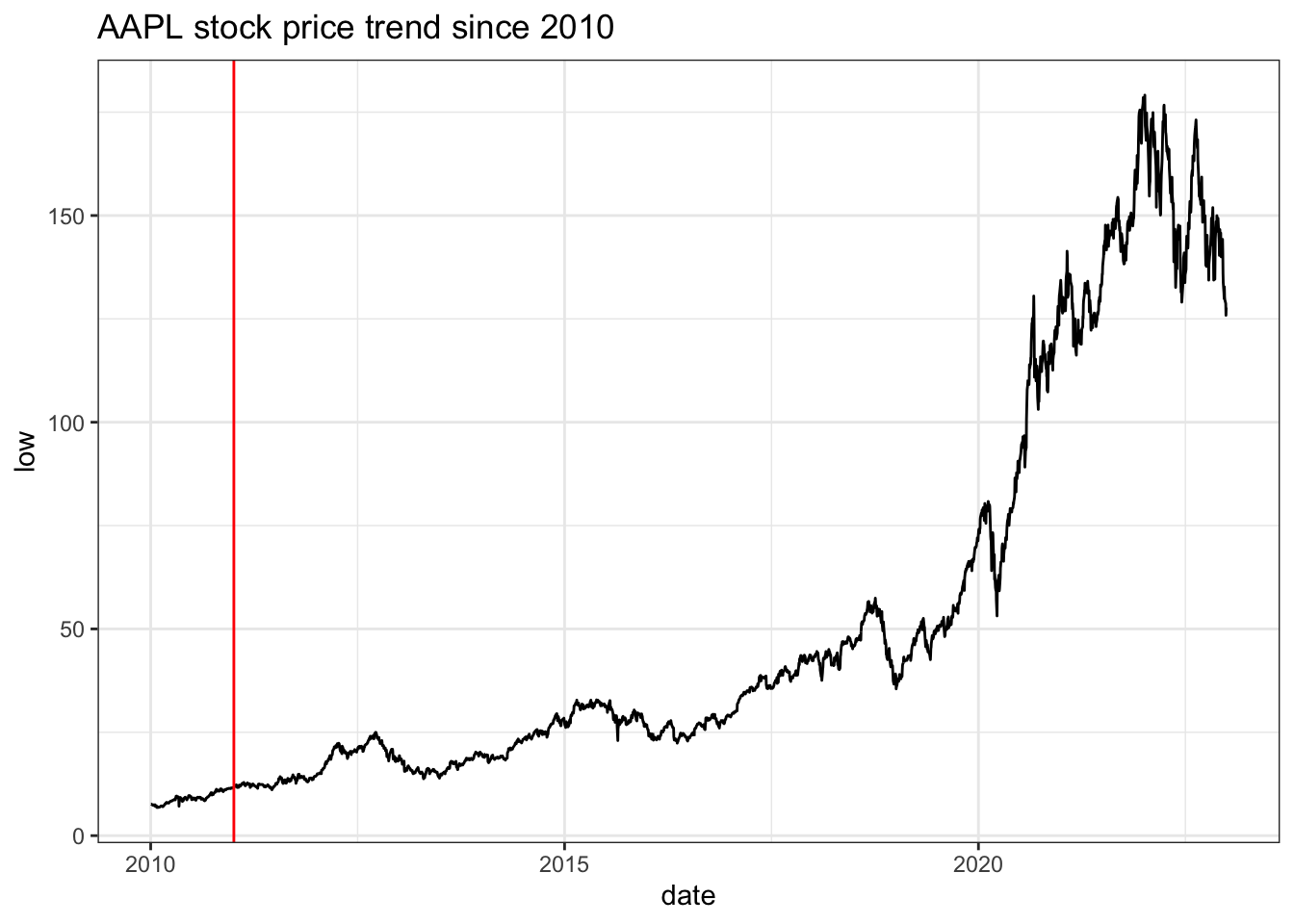

step 1: determine high and low point within period sliding window

First step is to find 52 week low and high for each date, and determine whether a given date is 52 week low/high or not.

determine_period_low_high calculate price of 52 week low and high for each date, and return Boolean values whether that date is 52 week low or high.

Code

determine_period_low_high <- function(df, period=354){
    
    stock_symbol <- df |>
        distinct(stock_symbol) |>
        pull(stock_symbol)
    
    wk52_low_high <- map_dfr(
        df$date,
        ~big_tech_stock_prices |> 
            filter(stock_symbol==!!stock_symbol, date <= .x, date > .x - period) |> 
            summarise(
                low_wk52 = min(low),
                high_wk52 = max(high)
            ) |> 
            mutate(date=.x)
    )
    
    df <- left_join(df, wk52_low_high) |> 
        mutate(
            is_wk52_low = ifelse(low==low_wk52, T, F),
            is_wk52_high = ifelse(high==high_wk52, T, F)
        )
    df
}

df <- determine_period_low_high(df)

Code

# plot whole time price trends with wk52_high (high) and wk52_low (red) point
big_tech_stock_prices |> 
    filter(stock_symbol==!!stock_symbol) |> 
    ggplot(aes(x = date, y = low)) +
    geom_line() +
    geom_vline(aes(xintercept = start_date), color = "red") +
    geom_point(
        data = df |> 
            filter(is_wk52_low),
        aes(color = is_wk52_low), shape = 3, color = "red") +
    geom_point(
        data = df |> 
            filter(is_wk52_high),
        aes(color = is_wk52_high), shape = 3, color = "blue")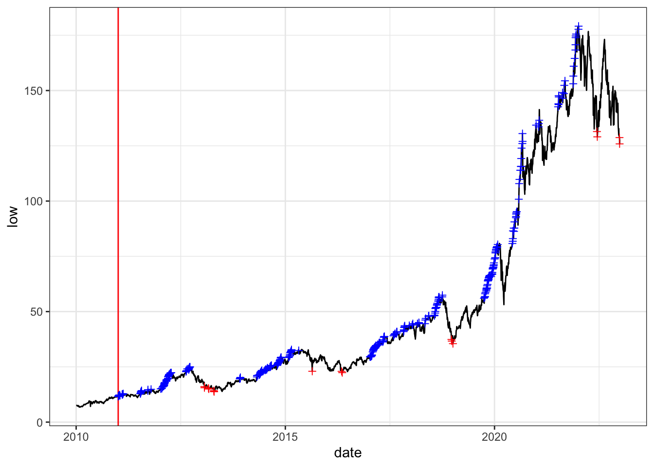

step 2: transaction date and price if have unlimited money

Even there are so many high and low points, since we sell everything at each transaction cycle, thus we can use first high point right after low points (buy points) to sell. If we have multiple low points in row, we will keep buying until we run out money.

To simplify the problem, we first assume we have unlimited cash, and determine buy and sell points from the high and low points.

determine_buy_sell_unlimited determine all possible buy and sell points when having unlimited cash.

Code

determine_buy_sell_unlimited <- function(df){
    # shorten df to have only possible low/high point and start with a wk52 low point
    df2 <- df |>
        filter(is_wk52_low | is_wk52_high) |>
        filter(cumsum(is_wk52_low) > 0)
    
    # create empty sell_df
    sell_df <- NULL
    
    # loop through df2 get all possible sell_df (since buy at all low points when with unlimited cash) - the first high after lows
    while(nrow(df2) > 0) {
        sell_df <- bind_rows(
            sell_df,
            df2 |>
                filter(cumsum(is_wk52_high) == 1) |> # the first high after lows
                select(stock_symbol, date, price = high)
        )
        
        df2 <- df2 |>
            filter(date > max(sell_df$date)) |>
            filter(cumsum(is_wk52_low) > 0) # shorten df2 to have only possible low/high point and start with next wk52 low point
        
        if (all(df2$is_wk52_low)) {
            break
        }
    }
    
    # create transaction_df by combining sell_df with buy_df
    transaction_df <- df |>
        filter(is_wk52_low) |>
        select(stock_symbol, date, price = low) |>
        mutate(transaction = "buy") |>
        bind_rows(sell_df |>
                      mutate(transaction = "sell")) |>
        arrange(date)
    
    # adding transaction cycle (using sell as end of one cycle)
    transaction_df <- transaction_df |>
        left_join(transaction_df |>
                      filter(transaction == "sell") |>
                      mutate(cycle = row_number())) |>
        fill(cycle, .direction = "up") |>
        group_by(cycle) |>
        mutate(cycle = cur_group_id()) |>
        ungroup()
    
    transaction_df
}

transaction_df <- determine_buy_sell_unlimited(df)

Code

# plot whole time price trends with transaction point
big_tech_stock_prices |> 
    filter(stock_symbol==!!stock_symbol) |> 
    ggplot(aes(x = date)) +
    geom_line(aes(y = low), color = "red", alpha = 0.2) +
    geom_line(aes(y = high), color = "blue", alpha = 0.2) +
    geom_vline(aes(xintercept = start_date), color = "orange") +
    geom_point(
        data = transaction_df,
        aes(y = price, color = transaction), shape = 3) +
    ggtitle(glue::glue("{stock_symbol} buy/sell opportunities"))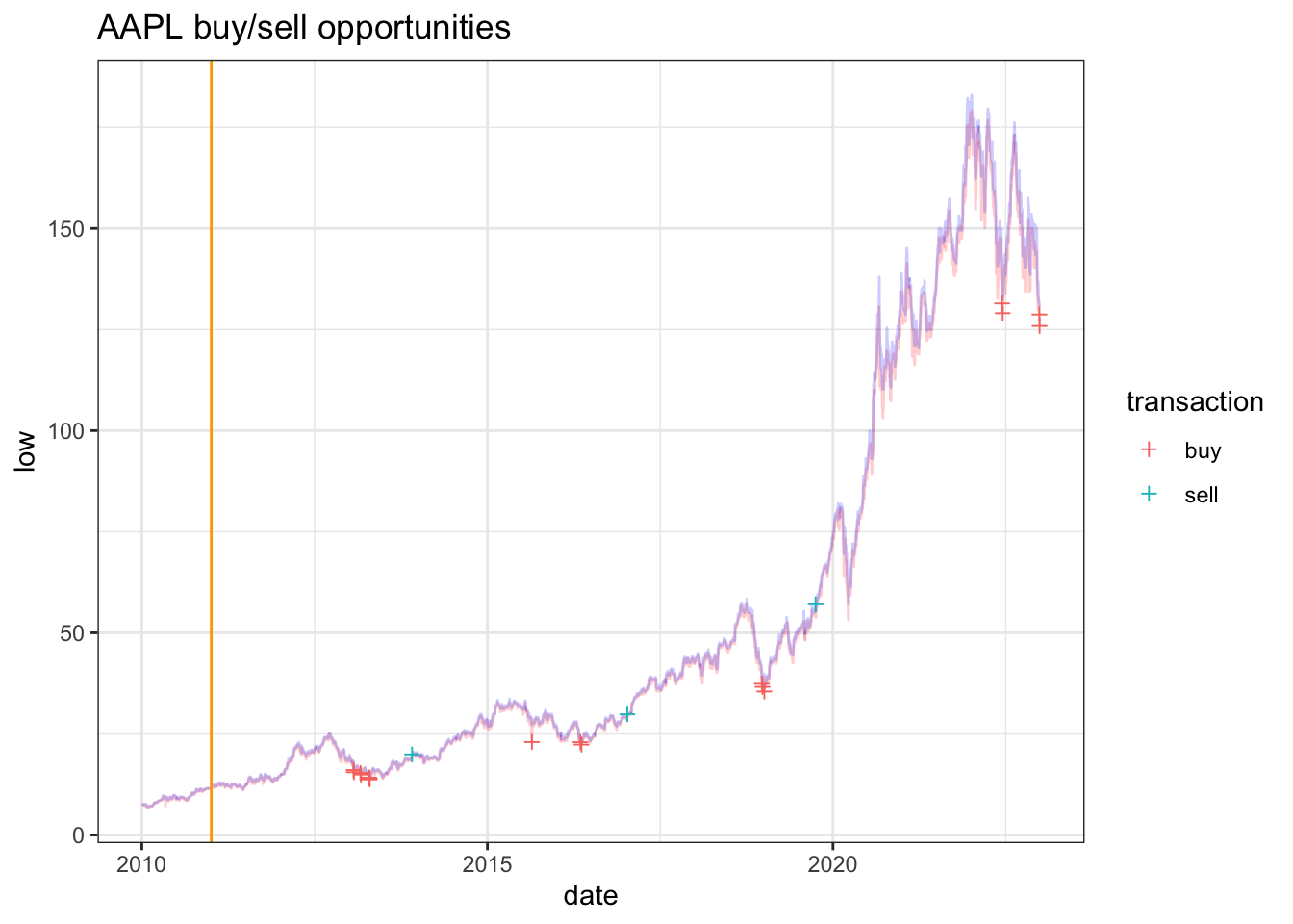

step 3: determine final sell/buy points and transaction details

The investment strategy (“buy low sell high”) have 4 options based on the different assumptions:

assuming you have unlimited of money, from the time ready to invest, always buy same number of stocks (num_per_buy) at 52 week low, and sell everything hold at 52 week high
assuming you have unlimited of money and you can buy stock bits (but have to sell as whole), from the time ready to invest, always spent same amount of cash (cash_per_buy) to buy at 52 week low, and sell everything hold at 52 week high.
assuming you have a fixed amount of money (total_cash), from the time ready to invest, always buy same number of stocks (num_per_buy) at 52 week low, and sell everything hold at 52 week high.
assuming you have a fixed amount of money (total_cash) and you can buy stock bits (but have to sell as whole), from the time ready to invest, always spent same amount of cash (cash_per_buy) to buy at 52 week low, and sell everything hold at 52 week high.

The transaction details include 1) how many stocks to buy/sell and 2) how much cash to spend/earn at each transaction. Depending on the invest options mentioned above, we create transaction detail for each option.

Note:

To simplify the problem, we always buy same number of stocks for option 3. If there is not enough, drop the whole buy transaction instead of buying smaller number of stocks.
Although stocks can be bought in bits but must be sold as whole.

buy_low_sell_high determine final transaction details.

Code

buy_low_sell_high <- function(transaction_df, cash_limit=Inf, num_per_buy, cash_per_buy=NULL){
    
    if(is.infinite(cash_limit)){
        # option 1: unlimited cash, buy whole stock with fixed number
        if(!is.null(num_per_buy)){
            buy_df <- transaction_df |>
                filter(transaction == "buy") |>
                mutate(stock_num = num_per_buy) |>
                mutate(stock_cash = -stock_num * price)
        # option 2: unlimited cash, buy bit stock with fixed cash
        }else if(!is.null(cash_per_buy)){
            buy_df <- transaction_df |>
                filter(transaction == "buy") |>
                mutate(stock_cash = -cash_per_buy) |>
                mutate(stock_num = -stock_cash / price)
        }
        
        # sell_df will be same for option 1 and option 2: at each cycle sell most whole stocks
        sell_df <- transaction_df |>
            filter(transaction == "sell") |>
            left_join(buy_df |>
                          group_by(cycle) |>
                          summarise(stock_num = -floor(sum(stock_num)))) |>  # can only sell whole stocks)
            mutate(stock_cash = -price * stock_num)
        
        transaction_df2 <- bind_rows(buy_df,
                                     sell_df) |>
            arrange(date) |>
            mutate(
                stock_num_cumsum = cumsum(stock_num),
                stock_cash_cumsum = cumsum(stock_cash)
            )
    }else{
        
        transaction_df2 <- NULL
        total_cash <- cash_limit
        # for each transaction cycle, has to cut off some buys to make sure stock_cash_cumsum > 0
        for (i in unique(transaction_df$cycle)) {
            # option 3: limited cash, buy whole stock with fixed number
            if(!is.null(num_per_buy)){
                buy_df <- transaction_df |>
                    filter(transaction == "buy", cycle == i) |>
                    mutate(stock_num = num_per_buy) |>
                    mutate(stock_cash = -stock_num * price) |>
                    mutate(
                        stock_num_cumsum = cumsum(stock_num),
                        stock_cash_cumsum = cumsum(stock_cash)
                    ) |>
                    mutate(stock_cash_cumsum = total_cash + stock_cash_cumsum) |>
                    filter(cumsum(stock_cash_cumsum >= 0) == row_number())
                
            # option 4: unlimited cash, buy bit stock with fixed cash
            }else if(!is.null(cash_per_buy)){
                buy_df <- transaction_df |>
                    filter(transaction == "buy", cycle == i) |>
                    mutate(stock_cash = -cash_per_buy) |>
                    mutate(stock_num = -stock_cash / price) |>
                    mutate(
                        stock_num_cumsum = cumsum(stock_num),
                        stock_cash_cumsum = cumsum(stock_cash)
                    ) |>
                    mutate(stock_cash_cumsum = total_cash + stock_cash_cumsum) |>
                    filter(cumsum(stock_cash_cumsum >= 0) == row_number())
            }
            
            
            if (nrow(buy_df) == 0) {
                break
            } else{
                sell_df <- transaction_df |>
                    filter(transaction == "sell", cycle == i) |>
                    left_join(buy_df |>
                                  group_by(cycle) |>
                                  summarise(stock_num = -floor(sum(stock_num)))) |>
                    mutate(stock_cash = -price * stock_num)
                
                transaction_df2 <- bind_rows(
                    transaction_df2,
                    bind_rows(buy_df,
                              sell_df) |>
                        arrange(date) |>
                        mutate(
                            stock_num_cumsum = cumsum(stock_num),
                            stock_cash_cumsum = total_cash + cumsum(stock_cash)
                        )
                )
                
                # update total cash after one cycle
                total_cash <-
                    transaction_df2 |> slice(n()) |> pull(stock_cash_cumsum)
            }
        }
    }
    transaction_df2
}

plot_transaction_details function plots details of transaction.

Code

plot_transaction_details <- function(transaction_df1, title) {
    stock_symbol <- unique(transaction_df1$stock_symbol)
    p1 <- big_tech_stock_prices |> 
        filter(stock_symbol==!!stock_symbol) |> 
    ggplot(aes(x = date)) +
    geom_line(aes(y = low), color = "red", alpha=0.2) +
    geom_line(aes(y = high), color = "blue", alpha=0.2) +
    geom_vline(aes(xintercept = start_date), color = "red") +
    geom_point(
        data = transaction_df1,
        aes(color = transaction, y=price), shape = 1) +
        ggtitle("Transaction history") +
        labs(y = 'Stock price') +
        theme(plot.title = element_text(face="bold",size=10))
    
    p2 <- big_tech_stock_prices |> 
        filter(stock_symbol==!!stock_symbol) |> 
        select(date) |> 
        left_join(
            transaction_df1
        ) |> 
        ggplot(aes(x=date, y = stock_num_cumsum)) +
        geom_point(aes(color = transaction), shape = 1) +
        geom_line(data = transaction_df1, linetype=3) +
        scale_colour_discrete(na.translate = F) +
        ggtitle("Stock number on holding") +
        labs(y = "Cumulative stock number")+
        theme(plot.title = element_text(face="bold",size=10))
    
    p3 <- big_tech_stock_prices |> 
        filter(stock_symbol==!!stock_symbol) |> 
        select(date) |> 
        left_join(
            transaction_df1
        ) |> 
        mutate(stock_cash_cumsum=ifelse(stock_cash_cumsum > 0, 0, stock_cash_cumsum)) |> 
        ggplot(aes(x=date, y = -stock_cash_cumsum)) +
        geom_point(aes(color = transaction), shape = 1) +
        geom_line(data = transaction_df1 |> 
    mutate(invested=ifelse(stock_cash_cumsum > 0, 0, -stock_cash_cumsum)) |> 
    mutate(gained=ifelse(stock_cash_cumsum < 0, 0, stock_cash_cumsum)) |> 
    select(date, invested, gained) |> 
    gather(-date, key="cash_type", value = "cash"), aes(y=cash, linetype=cash_type)) +
        geom_point(data = transaction_df1 |> 
    mutate(gained=ifelse(stock_cash_cumsum < 0, 0, stock_cash_cumsum)), aes(y=gained, color = transaction), shape=1) + 
        scale_colour_discrete(na.translate = F) +
        ggtitle("Investment and gain in total") +
        labs(y = "Invested or gained cash")+
        theme(plot.title = element_text(face="bold",size=10))
    
    
    tmp <- transaction_df1 |> 
        filter(transaction=="buy") |> 
        select(buy_date=date, cycle, buy_stock=stock_num) |> 
        left_join(
            transaction_df1 |> 
                filter(transaction=="sell") |> 
                select(sell_date=date, cycle, sell_stock=stock_num_cumsum)
        ) |> 
        filter(!is.na(sell_date)) |> 
        group_by(cycle) |> 
        mutate(stock_num = ifelse(
            row_number()==n(), buy_stock-sell_stock, buy_stock
        )) |> 
        ungroup() |> 
        mutate(stock_age = as.integer(sell_date-buy_date))
 
    p4 <- tmp |> 
        left_join(
            tmp |> 
                group_by(cycle) |> 
                summarise(
                    cycle_dates = glue::glue("{as.character(min(buy_date))}~\n {as.character(max(sell_date))}")
                ) |> 
                ungroup()
        ) |> 
        ggplot(aes(y = cycle_dates)) +
        geom_point(aes(x=stock_age, size=stock_num), alpha=0.2, color="red", shape=1) +
        geom_point(data = tmp |> 
        group_by(cycle) |> 
        summarise(stock_cycle_age = sum(stock_age*stock_num)/sum(stock_num),
                  cycle_dates = glue::glue("{as.character(min(buy_date))}~\n {as.character(max(sell_date))}")), aes(x = stock_cycle_age), shape=3, color="red") +
        ggrepel::geom_text_repel(data = tmp |> 
        group_by(cycle) |> 
        summarise(stock_cycle_age = sum(stock_age*stock_num)/sum(stock_num),
                  cycle_dates = glue::glue("{as.character(min(buy_date))}~\n {as.character(max(sell_date))}")), aes(x = stock_cycle_age, label = as.integer(stock_cycle_age)), color="red") +
        ggtitle("Stock investment length") +
        labs(x = "stock age", y = "")+
        theme(plot.title = element_text(face="bold",size=10))
   
    p <- cowplot::plot_grid(p1, p2, p3, p4, nrow = 2)
    
    cowplot::plot_grid(
    ggplot() + ggtitle('option 2: unlimited cash, buy bit stock with fixed cash') + theme(plot.title = element_text(face="bold",size=12)),
    p,
    ncol = 1,
    rel_heights = c(0.06, 1)
)
    
}

To make options comparable across, we set cash_limit as 1000, num_per_buy as 10 and cash_per_buy as 1000, and being consistent across all the options and stocks.

cash_limit <- 1000
num_per_buy <- 10
cash_per_buy <- 1000

option 1: unlimited cash, buy whole stock with fixed number

transaction_df1 <- buy_low_sell_high(transaction_df, cash_limit=Inf, num_per_buy=num_per_buy, cash_per_buy=NULL)

Code

plot_transaction_details(transaction_df1,
                         title = 'option 1: unlimited cash, buy whole stock with fixed number')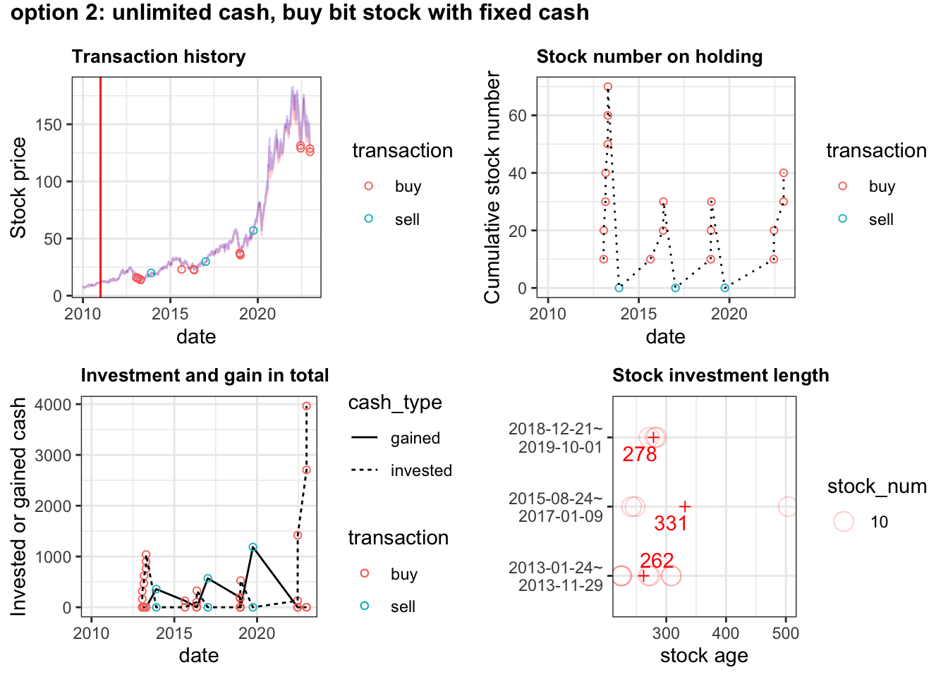

option 2: unlimited cash, buy bit stock with fixed cash

transaction_df2 <- buy_low_sell_high(transaction_df, cash_limit=Inf, num_per_buy=NULL, cash_per_buy=cash_per_buy)

Code

plot_transaction_details(transaction_df2,
                         title = 'option 2: unlimited cash, buy bit stock with fixed cash')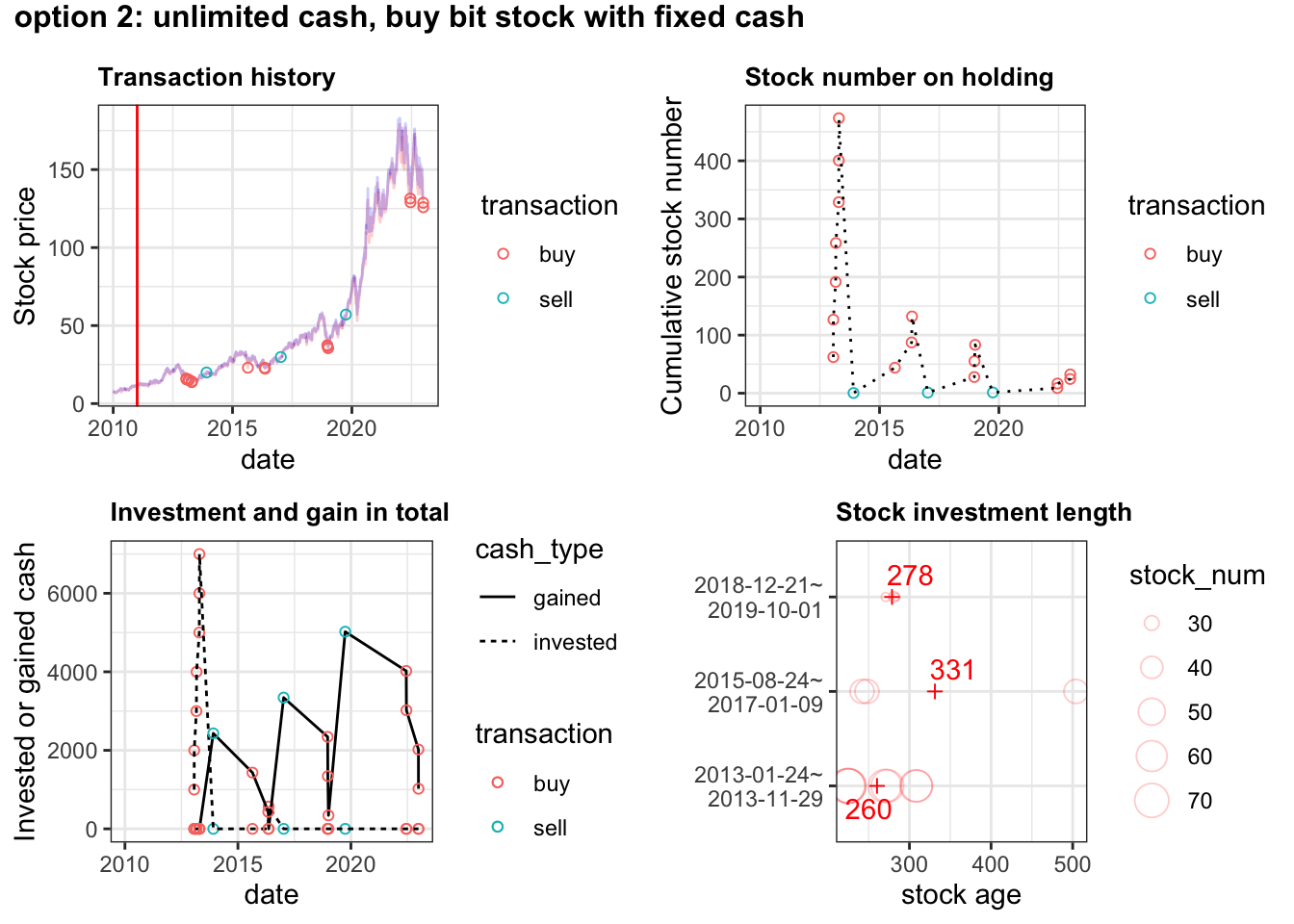

option 3: limited cash, buy whole stock with fixed number

transaction_df3 <- buy_low_sell_high(transaction_df, cash_limit=cash_limit, num_per_buy=num_per_buy, cash_per_buy=NULL)

Code

plot_transaction_details(transaction_df3,
                         title = 'option 3: limited cash, buy whole stock with fixed number')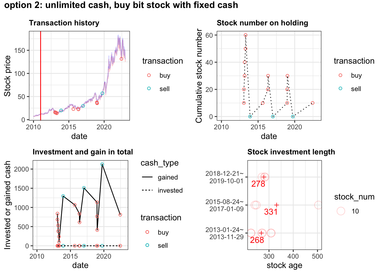

option 4: unlimited cash, buy bit stock with fixed cash

transaction_df4 <- buy_low_sell_high(transaction_df, cash_limit=cash_limit, num_per_buy=NULL, cash_per_buy=cash_per_buy)

Code

plot_transaction_details(transaction_df4,
                         title = 'option 4: unlimited cash, buy bit stock with fixed cash')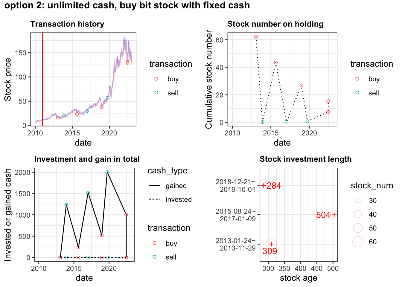

Which option is better?

To determine which option is better, we have to evaluate investment outcome by gain-risk ratio. The simple gain-risk ratio can be estimated by the earned cashed divided by required input.

Code

eval_df <- left_join(
    # stock_cash_cumsum reported for all options
    list(transaction_df1,
         transaction_df2,
         transaction_df3,
         transaction_df4) |>
        map_dfr(~ .x |>
                    filter(transaction == "sell") |>
                    slice(n()) |>
                    select(stock_cash_cumsum)) |>
        mutate(option = row_number()) |>
        mutate(option = glue::glue("option_{option}")),
    
    # required_input money
    list(transaction_df1,
         transaction_df2) |>
        map_dfr( ~ .x |>
                     slice(1:max(which(stock_num < 0))) |>
                     filter(stock_cash_cumsum < 0) |> 
                     summarise(required_input = max(abs(stock_cash_cumsum)))) |> 
    mutate(option = row_number()) |> 
    mutate(option = glue::glue("option_{option}"))
) |> 
    mutate(money_gain = ifelse(is.na(required_input), stock_cash_cumsum-cash_limit, stock_cash_cumsum)) |> # the last stock_cash_cumsum include the input cash in option 3/4
    mutate(required_input=ifelse(is.na(required_input), cash_limit, required_input)) |> 
    select(-stock_cash_cumsum)

eval_df |> 
    mutate(gain_risk_ratio = money_gain/required_input) |> 
    mutate(gain_risk_ratio = scales::percent(gain_risk_ratio)) |> 
    mutate_at(c("required_input", "money_gain"), ~gsub("^", "$", format(.x, digits=2, big.mark=","))) |> 
    dplyr::rename(" "=1, "maximun investment"=2, "total gain"=3, "gain %"=4) |> 
    knitr::kable(caption = "Gain-risk ratio for buy-low-sell-high options", align="c")

Gain-risk ratio for buy-low-sell-high options
	maximun investment	total gain	gain %
option_1	$1,038	$1,186	114.2%
option_2	$7,000	$5,022	71.7%
option_3	$1,000	$1,124	112.4%
option_4	$1,000	$1,004	100.4%

For APPL, it seems buy same whole stock each buy is better strategy than spending fixed money at 52 week low. If you cannot get more than $1000, option 3 – with limited cash (only $1000), buy whole stock with fixed number –is the best strategy. It took least amount of input money (low risk) to get reasonable gain.

Which big tech gave best gain using buy-low-sell-high option 3?

Above we use Apple stock (APPL) as an example, from the earliest available date, observe for one period (52 weeks), then ready to invest.

cash_limit <- 1000
num_per_buy <- 10
cash_per_buy <- 1000
period <- 364

df_all_tech <- big_tech_stock_prices |> 
            group_by(stock_symbol) |> 
            slice(which.min(date)) |> 
            ungroup() |> 
            select(stock_symbol, start_date=date) |> 
            left_join(
                big_tech_stock_prices
            ) |> 
            filter(date >= start_date + period) |> 
            select(-start_date)

df_all_tech <- split(df_all_tech, df_all_tech$stock_symbol)


transaction_df_all_tech <-
    map_dfr(names(df_all_tech),
            function(tech_symbol) {
                cat(paste("START", tech_symbol, "\n"))
                df <- df_all_tech[[tech_symbol]]
                cat("run determine_period_low_high...\n")
                step1_df <- determine_period_low_high(df)
                cat("run determine_buy_sell_unlimited...\n")
                step2_transaction_df <-
                    determine_buy_sell_unlimited(step1_df)
                cat("run buy_low_sell_high...")
                buy_low_sell_high(
                    step2_transaction_df,
                    cash_limit = cash_limit,
                    num_per_buy = num_per_buy,
                    cash_per_buy = NULL
                )
            })

Thanks to Tanya Shapiro, I will add the company logos curated by her to the plot ².

Code

base_url <- "https://raw.githubusercontent.com/tashapiro/TidyTuesday/master/2023/W6/logos/"


tmp <- transaction_df_all_tech |> 
    filter(transaction=="sell") |> 
    group_by(stock_symbol) |> 
    slice(n()) |> 
    select(stock_symbol, stock_cash_cumsum) |> 
    mutate(money_gain = stock_cash_cumsum-1000) |> 
    ungroup()

# logos <- glue::glue("<img src='{base_url}{tmp$stock_symbol}.png' width='25' /><br>{tmp$stock_symbol}") |> as.character()
# names(logos) <- tmp$stock_symbol

tmp |> 
    mutate(logo = glue::glue("{base_url}{tmp$stock_symbol}.png")) |> 
    ggplot(aes(x = money_gain, y = fct_reorder(stock_symbol, money_gain))) +
    geom_col(fill="skyblue") +
    labs(x = "US dollars", y="") +
    ggtitle("Amount of gain the with $1000 investment") +
    ggimage::geom_image(aes(x = 0, image=logo))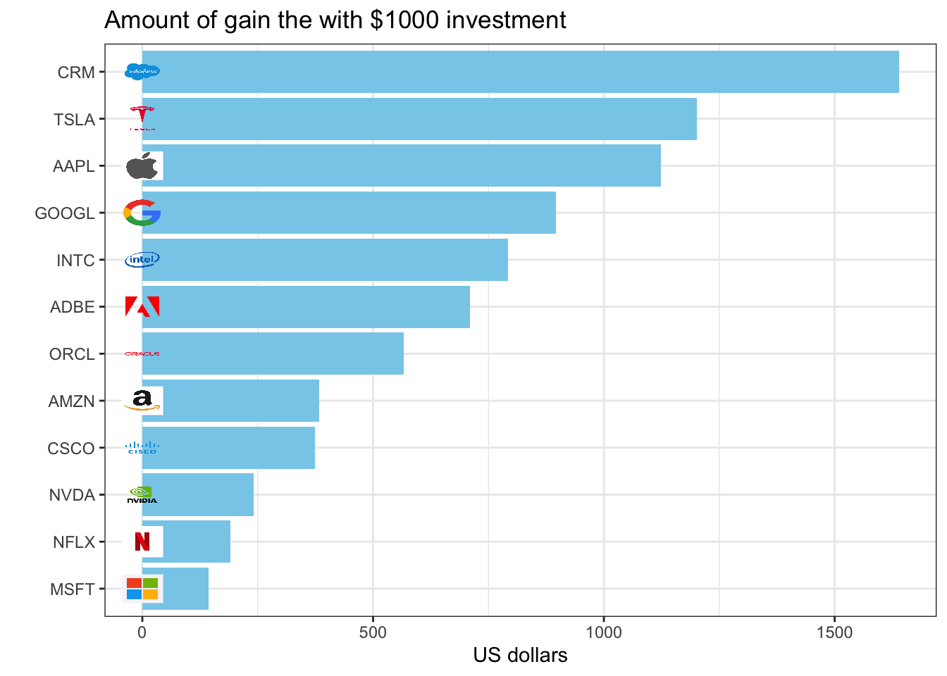

Note: The reason “META” and “IBM” failed to show because they were too expensive to buy at their first 52 weeks low (10 stocks were already beyond my cash limit)!!!

Final thoughts

Due to the time limit, I will end this TidyTuesday exercise here. However, there are till many interesting ideas to explore.

If we adjust parameters in the “buy-low-sell-high” strategy, eg: start_date, period, cash_limit, num_per_buy and cash_per_buy, will it make gain-risk-ratio change dramatically within the same stock? Just like I tune hyper-parameters in ML exercise!
The current model did not take taxes (which is a big expense in trading) into consideration. How long to hold a stock determines tax brackets. It will improve the estimate accuracy of true gain.
All the price of big tech stocks were slowly climbing up at early time. Will my functions break if the stock kept dropping?
All the price of big tech stocks are quite stable. Will a more fluctuated stock make difference on the “buy-low-sell-high” strategy?
I did not use this strategy in my personal trading. Instead, I just invest fixed amount of cash into index fund recurrently with a certain frequency. How about writing the “recurrent invest” strategy and comparing this to “buy-low-sell-high” strategy?

At R-ladies Philly event, Alice mentioned a R package {quantmod} to download daily price for any stocks and perform quantitative financial modeling. I may want to try it out sometime.

Besides the stock context itself, I have a few final take-away from this exercise:

When question is complicated, I should modularize the question and solve the big question by accomplishing little steps first.

Modular programming is one-step towards object-oriented programming, although there are difference between modular programming and object-oriented programming ³.
I had to spend an extra night to clean up the code to make everything function-based (object-oriented?). However, just like writing paper, spitting it out is always the hardest but also the very first step. Do not worry about the coding style at beginning, just spit it out!

As usually, I picked up several tricks to “filter” the rows.

using filter(cumsum(<boolean>) ...)
- filter(cumsum(is_wk52_low) > 0): remove the first x rows where is_wk52_low is FALSE (but not removing anything after is_wk52_low being TRUE once)
- filter(cumsum(is_wk52_high) == 1): remove everything after is_wk52_high is TRUE for the first time
- filter(cumsum(stock_cash_cumsum >= 0) == row_number()): remove everything after stock_cash_cumsum >= 0 is FALSE for the first time (note: different from simple filter(stock_cash_cumsum >=0) by even removing stock_cash_cumsum >=0 cases after first FALSE case)
using slice()
- slice(n()): just keep last row
- slice(1:max(which(stock_num < 0))): keep first row until the last row where stock_num < 0

Footnotes

Thomas Mock (2022). Tidy Tuesday: A weekly data project aimed at the R ecosystem. https://github.com/rfordatascience/tidytuesday.↩︎
I tried to put logo in y axis using ggtext like this, but I kept getting “libpng error: Not a PNG file ggtext”.↩︎
What is the big difference between modular and object oriented programming?↩︎