TidyTuesday: predict chocolate rating with xgboost

Load required libraries

Code

library(tidyverse)
library(tidymodels)
# library(lubridate)
library(vip)

Data README is available at here.

Clean Data

Code

chocolate_raw <- tuesdata$chocolate
chocolate_raw <- chocolate_raw %>% 
    mutate(cocoa_percent = parse_number(cocoa_percent)) %>% 
    separate(ingredients, c("ingredient_num","ingredients"), sep="-") %>% 
    mutate(
        ingredient_num=parse_number(ingredient_num),
        ingredients=str_trim(ingredients)
    ) %>% 
    mutate(ingredients = map(ingredients, ~str_split(.x, ",")[[1]])) %>% 
    mutate(most_memorable_characteristics=map(most_memorable_characteristics, ~str_split(.x,",")[[1]])) %>% 
    mutate(most_memorable_characteristics=map(most_memorable_characteristics, ~str_trim(.x))) %>% 
    # select(cocoa_percent, ingredient_num, ingredients, most_memorable_characteristics) %>%
    I()

• Convert gredients to boolean columns

using unnest to spread out the list column ingredients.

Code

gredients <- chocolate_raw %>% 
    mutate(line_n = row_number()) %>% 
    select(line_n, ingredients) %>% 
    unnest(cols=c(ingredients)) %>% 
    mutate(tmp=1) %>% 
    pivot_wider(names_from=ingredients, values_from=tmp) %>% 
    select(-"NA") %>% 
    janitor::clean_names() %>% 
    mutate_at(vars(-line_n), ~ifelse(is.na(.x),0,.x)) %>% 
    I()

• Convert most_memorable_characteristics to boolean columns

Code

most_memorable_characteristics <- chocolate_raw %>% 
    mutate(line_n = row_number()) %>% 
    select(line_n, most_memorable_characteristics) %>% 
    unnest(cols=c(most_memorable_characteristics)) %>% 
    mutate(tmp=1) %>% 
    # distinct(most_memorable_characteristics) %>% 
    # pivot_wider(names_from=most_memorable_characteristics, values_from=tmp) %>% 
    I()

There are 972 most_memorable_characteristics in total

Code

most_memorable_characteristics %>% 
    # mutate(most_memorable_characteristics = fct_lump_min(most_memorable_characteristics, min=100)) %>% 
    group_by(most_memorable_characteristics) %>% 
    count(sort=T) %>% 
    head(20) %>% 
    ggplot(aes(x=n, y=reorder(most_memorable_characteristics,n))) +
    geom_col() +
    geom_text(aes(label=n), color="white", hjust=1) +
    theme_bw() +
    labs(x="# of chocolates", y="most memorable characteristics")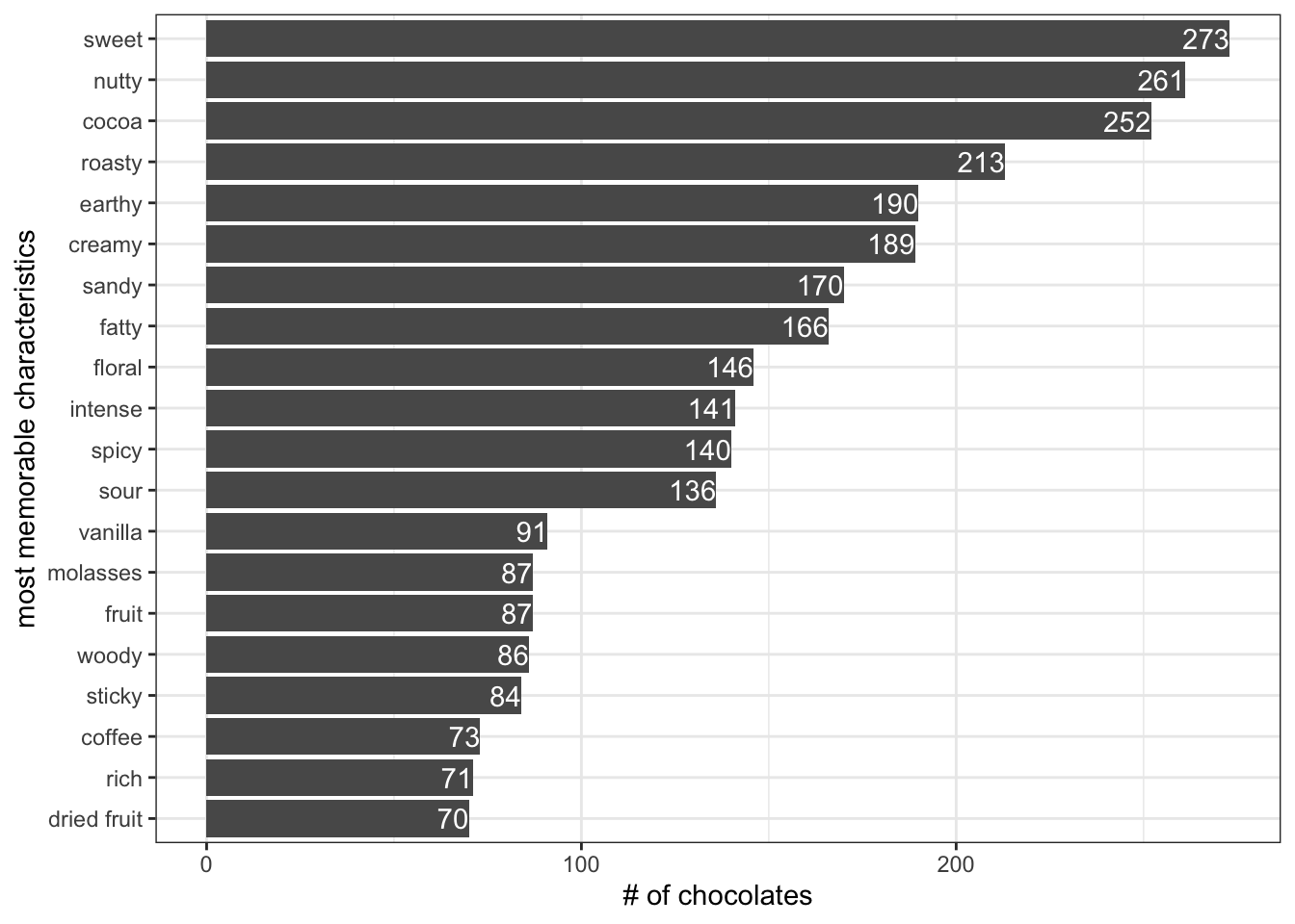

Pick top 12 most_memorable_characteristics to convert to boolean column

Code

most_memorable_characteristics <- most_memorable_characteristics %>% 
    mutate(most_memorable_characteristics = fct_lump_min(most_memorable_characteristics, min=100)) %>% 
    distinct() %>% 
    pivot_wider(names_from=most_memorable_characteristics, values_from=tmp) %>% 
    mutate_at(vars(-line_n), ~ifelse(is.na(.x),0,.x))

• create chocolate_clean data

Code

chocolate_clean <-
    chocolate_raw %>% 
    mutate(line_n=row_number()) %>% 
    select(-ingredients, -most_memorable_characteristics) %>% 
    left_join(gredients) %>%
    left_join(most_memorable_characteristics) %>%
    I()

Explore Data

Several features are explored in terms of their association with rating.

• country_of_bean_origin

Code

chocolate_clean %>% 
    mutate(country_of_bean_origin = fct_lump(country_of_bean_origin, n=10)) %>% 
    ggplot(aes(x=rating, y=country_of_bean_origin)) +
    geom_boxplot(aes(fill=country_of_bean_origin)) +
    theme_bw()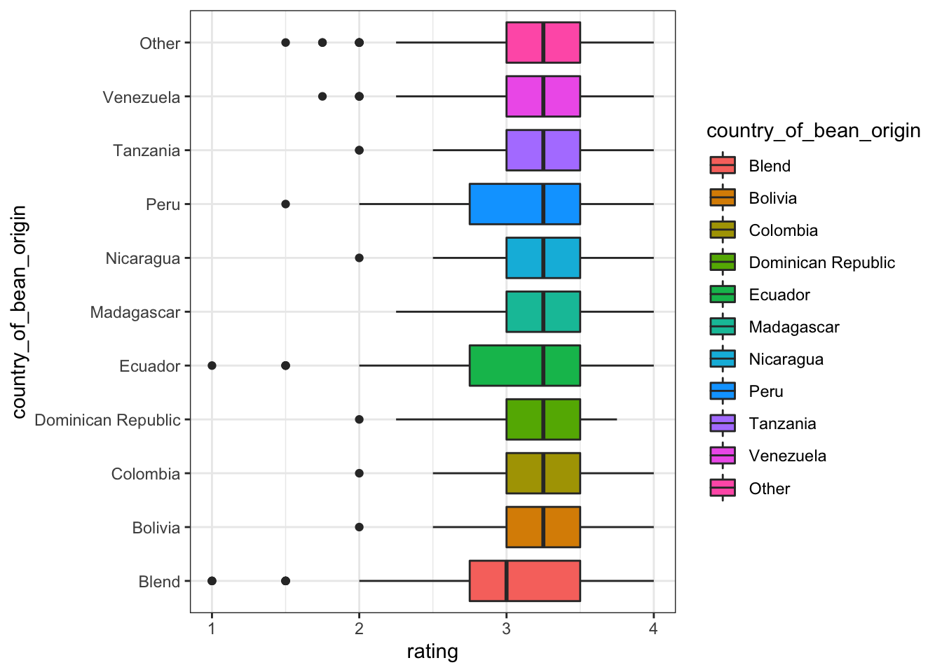

Blend and non-blend on country_of_bean_origin shows big difference, thus we convert country_of_bean_origin to country_of_bean_origin_blend

Code

chocolate_clean <- chocolate_clean %>% 
    mutate(country_of_bean_origin_blend = ifelse(country_of_bean_origin=="Blend", country_of_bean_origin, "Non-blend"))

• company_manufacturer and company_location

Code

chocolate_clean %>% 
    mutate(company_manufacturer = fct_lump(company_manufacturer, prop=0.01)) %>% 
    ggplot(aes(x=rating, y=reorder(company_manufacturer, rating, median))) +
    geom_boxplot(aes(fill=company_manufacturer)) +
    theme_bw() +
    labs(y="company_manufacturer")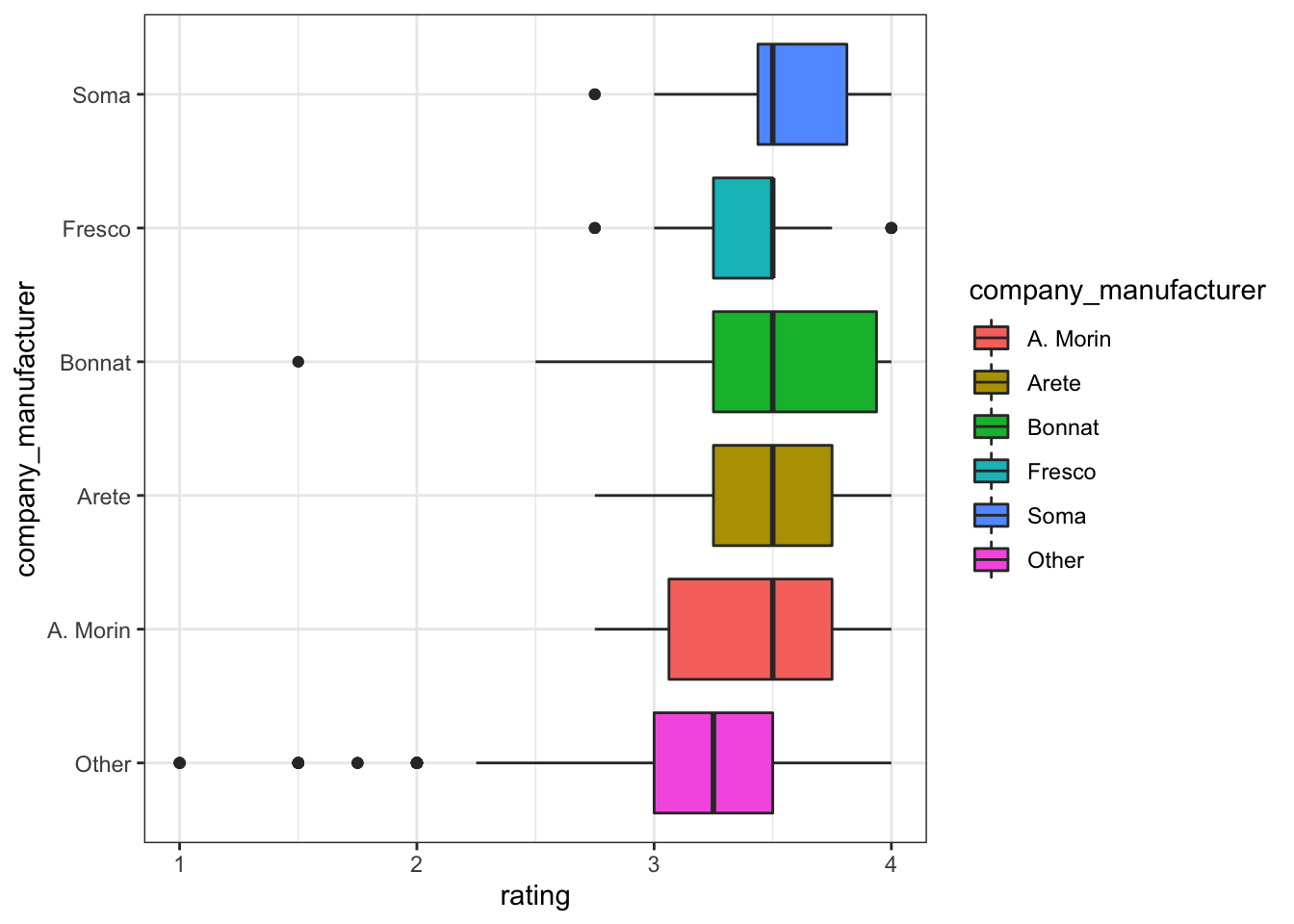

Code

chocolate_clean %>% 
    mutate(company_location = fct_lump(company_location, n=5)) %>% 
    ggplot(aes(x=rating, y=reorder(company_location, rating))) +
    geom_boxplot(aes(fill=company_location)) +
    theme_bw() +
    labs(y="company_location")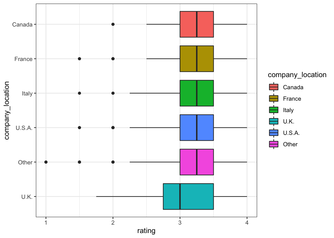

• cocoa_percent

Code

chocolate_clean %>% 
    ggplot(aes(x=cocoa_percent, y=rating)) +
    geom_point(aes(color=as.factor(cocoa))) +
    theme_bw() +
    theme(legend.position = "bottom") +
    labs(color="cocoa as most_memorable_characteristics")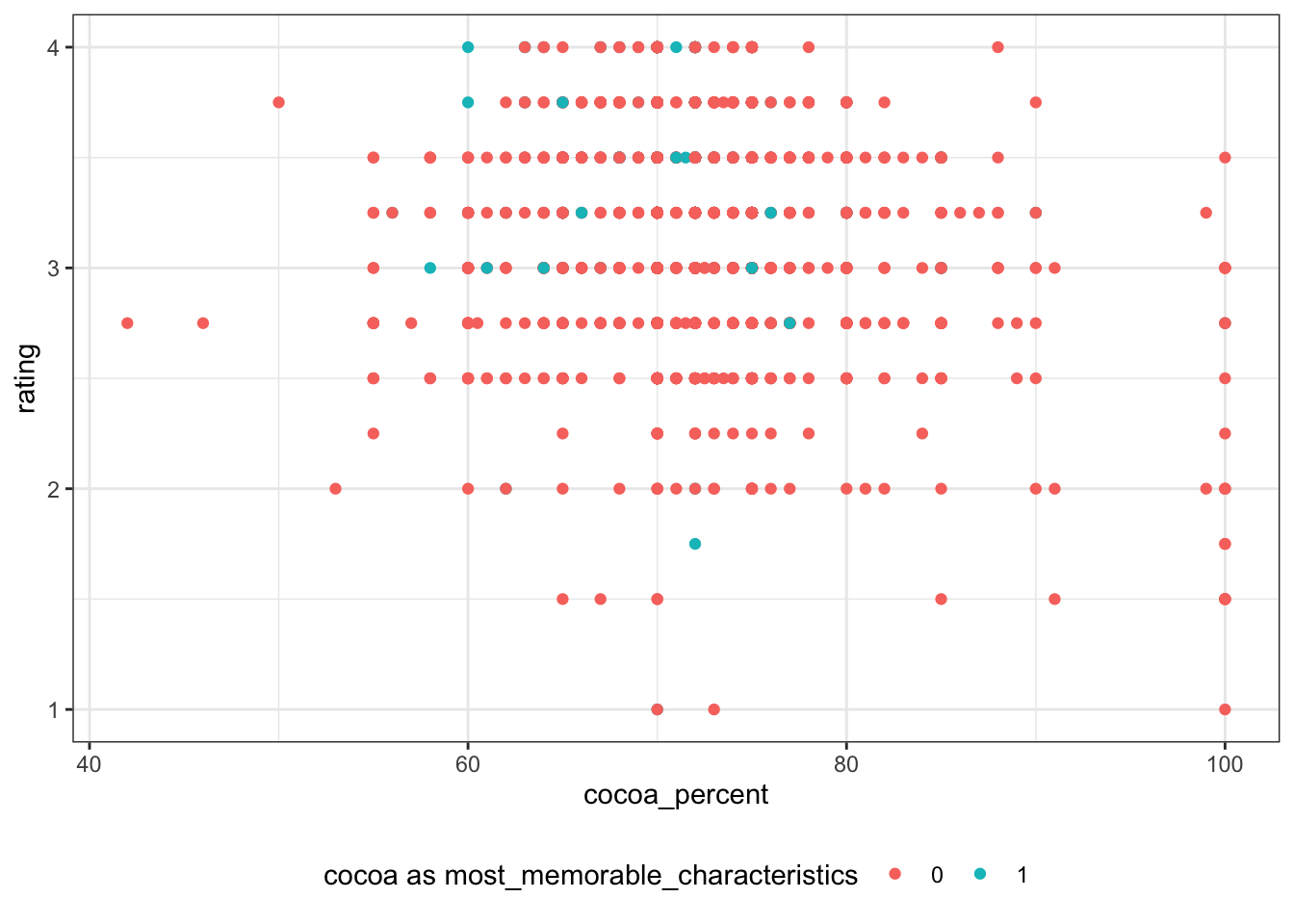

rating is not as continuous as what i originally imagined. Thus, I convert rating to nominal variable rating_bl using 3 as threshold

Code

chocolate_clean <- chocolate_clean %>% 
    mutate(rating_bl = ifelse(rating >= 3, ">=3", "< 3"))

chocolate_clean %>% 
    group_by(rating_bl) %>% 
    count()

# A tibble: 2 × 2
# Groups:   rating_bl [2]
  rating_bl     n
  <chr>     <int>
1 < 3         566
2 >=3        1964

Code

chocolate_clean %>% 
    ggplot(aes(x=cocoa_percent, y=rating_bl)) +
    geom_boxplot(aes(fill=as.factor(cocoa))) +
    theme_bw() +
    labs(y="rating", fill="cocoa as most_memorable_characteristics") +
    theme(legend.position = "bottom")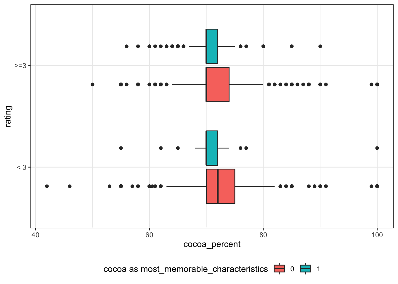

• most_memorable_characteristics

Code

chocolate_clean <- chocolate_clean %>% 
    mutate_at(vars(Other:creamy), as.factor)

most_memorable_characteristics like cocoa and creamy positive effect rating, while fatty, earthy, sandy, sour and sweet negatively effect rating.

Code

chocolate_clean %>% 
    select(rating, fatty:creamy) %>% 
    pivot_longer(!rating, names_to="most_memorable_characteristics", values_to="yes") %>%
    ggplot(aes(y=reorder(most_memorable_characteristics, rating, FUN=median), x=rating)) +
    geom_boxplot(aes(fill=yes)) +
    theme_bw() +
    theme(
        legend.position = "bottom"
    ) +
    scale_fill_discrete(labels = c("0"="No", "1"="Yes")) +
    labs(y="most_memorable_characteristics", fill="is most_memorable_characteristics?") +
    NULL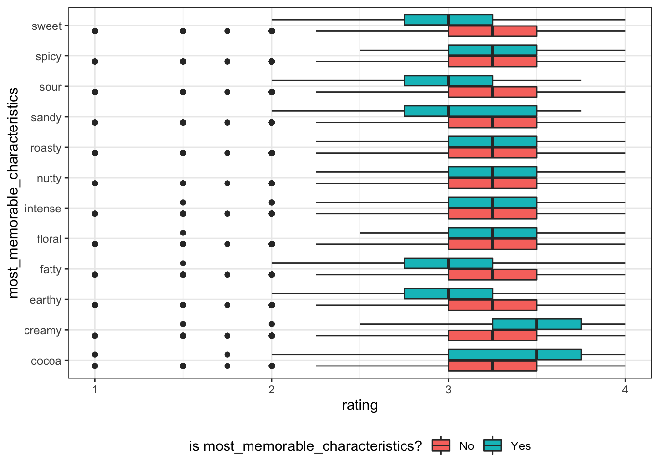

• ingredients

Code

chocolate_clean <- 
    chocolate_clean %>% 
    dplyr::rename(igrdt_beans=b, igrdt_sugar=s, igrdt_cocoa=c, igrdt_lecithin=l, igrdt_vanilla=v, igrdt_salt=sa, igrdt_sweeter=s_2) %>% 
    mutate_at(vars(contains("igrdt_")), as.factor)

ingredient number ingredient_num between 2-3 are associated with higher rating.

Code

chocolate_clean %>% 
    mutate(ingredient_num=as.factor(ingredient_num)) %>% 
    filter(!is.na(ingredient_num)) %>% 
    ggplot(aes(x = ingredient_num, y=rating)) +
    geom_boxplot()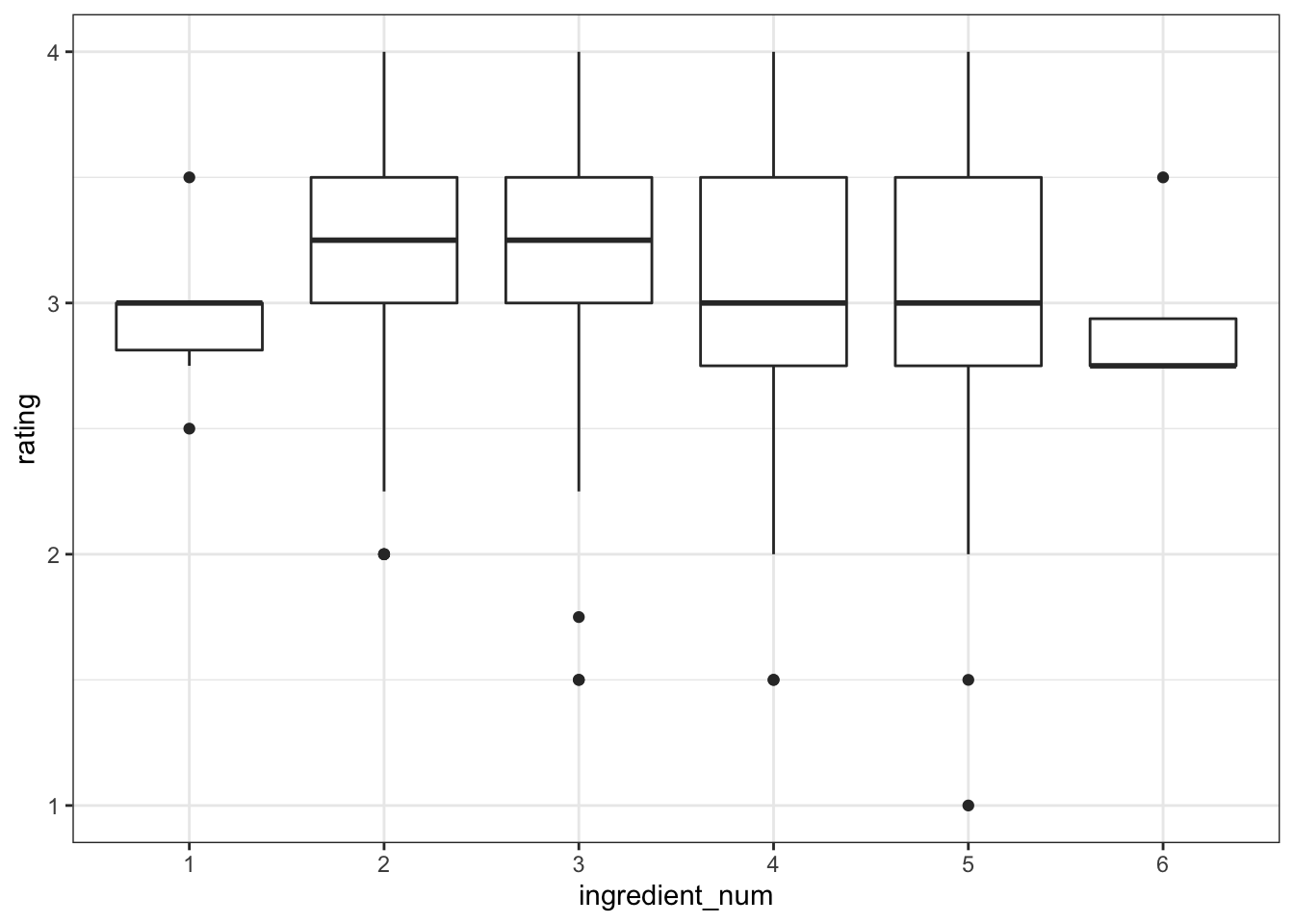

ingrediants like beans and sugar positively effect rating, while vanilla, sweeter and salt negatively effect rating.

Code

chocolate_clean %>% 
    select(rating, contains("igrdt_")) %>% 
    pivot_longer(!rating, names_to="ingredients", values_to="yes") %>%
    mutate(ingredients = gsub("igrdt_","",ingredients)) %>% 
    ggplot(aes(y=reorder(ingredients, rating, FUN=median), x=rating)) +
    geom_boxplot(aes(fill=yes)) +
    theme_bw() +
    theme(
        legend.position = "bottom"
    ) +
    scale_fill_discrete(labels = c("0"="No", "1"="Yes")) +
    labs(y="ingredients", fill="contain the ingredient?") +
    NULL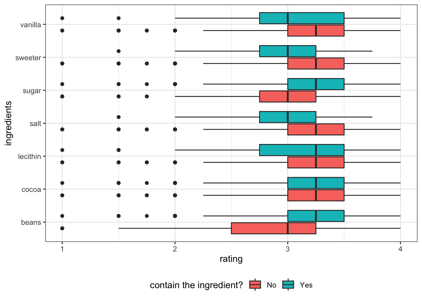

ML

Based on the exploratory analysis, to study the effect on overall rating of chocolates, the following features are selected for building ML models. Plus, using nominal feature rating_bl instead of numeric feature rating as outcome.

Code

chocolate_df <- chocolate_clean %>% 
    select(rating_bl, company_manufacturer, country_of_bean_origin_blend, cocoa_percent, ingredient_num, contains('igrdt_'), cocoa, creamy, fatty, earthy, sandy, sour, sweet) %>% 
    select(-igrdt_cocoa, -igrdt_lecithin) %>% 
    na.omit()

split samples

• initial_split

Code

set.seed(123)
chocolate_split <- initial_split(chocolate_df, strata = rating_bl)
chocolate_train <- training(chocolate_split)
chocolate_testing <- testing(chocolate_split)

• resample

Code

set.seed(123)
folds <- vfold_cv(chocolate_train, v = 10)
folds

#  10-fold cross-validation 
# A tibble: 10 × 2
   splits             id    
   <list>             <chr> 
 1 <split [1647/184]> Fold01
 2 <split [1648/183]> Fold02
 3 <split [1648/183]> Fold03
 4 <split [1648/183]> Fold04
 5 <split [1648/183]> Fold05
 6 <split [1648/183]> Fold06
 7 <split [1648/183]> Fold07
 8 <split [1648/183]> Fold08
 9 <split [1648/183]> Fold09
10 <split [1648/183]> Fold10

recipe

Code

chocolate_rec <- 
    recipe(rating_bl ~ ., data = chocolate_train) %>% 
    step_other(company_manufacturer, threshold=0.01, other="otherCompany") %>% 
    # step_mutate_at(c("company_manufacturer","country_of_bean_origin_blend", "rating_bl"), fn = ~as.factor(.x)) %>% 
    step_dummy(all_nominal_predictors()) %>% 
    step_zv(all_predictors())

chocolate_rec

Recipe

Inputs:

      role #variables
   outcome          1
 predictor         16

Operations:

Collapsing factor levels for company_manufacturer
Dummy variables from all_nominal_predictors()
Zero variance filter on all_predictors()

check preprocessed data.frame

Code

chocolate_rec %>% 
    prep(new_data = NULL) %>% 
    juice()

# A tibble: 1,831 × 20
   cocoa_percent ingre…¹ ratin…² compa…³ compa…⁴ compa…⁵ compa…⁶ compa…⁷ count…⁸
           <dbl>   <dbl> <fct>     <dbl>   <dbl>   <dbl>   <dbl>   <dbl>   <dbl>
 1            70       4 < 3           0       0       0       0       0       1
 2            70       4 < 3           0       0       0       0       0       1
 3            60       3 < 3           0       0       0       0       1       1
 4            70       2 < 3           0       0       0       0       1       1
 5            70       2 < 3           0       0       0       0       1       1
 6            75       4 < 3           0       0       0       0       1       1
 7            75       4 < 3           0       0       0       0       1       1
 8            75       5 < 3           0       0       0       0       1       1
 9            75       5 < 3           0       0       0       0       1       1
10            65       6 < 3           0       0       0       0       1       1
# … with 1,821 more rows, 11 more variables: igrdt_sugar_X1 <dbl>,
#   igrdt_vanilla_X1 <dbl>, igrdt_salt_X1 <dbl>, igrdt_sweeter_X1 <dbl>,
#   cocoa_X1 <dbl>, creamy_X1 <dbl>, fatty_X1 <dbl>, earthy_X1 <dbl>,
#   sandy_X1 <dbl>, sour_X1 <dbl>, sweet_X1 <dbl>, and abbreviated variable
#   names ¹​ingredient_num, ²​rating_bl, ³​company_manufacturer_Arete,
#   ⁴​company_manufacturer_Bonnat, ⁵​company_manufacturer_Fresco,
#   ⁶​company_manufacturer_Soma, ⁷​company_manufacturer_otherCompany, …
# ℹ Use `print(n = ...)` to see more rows, and `colnames()` to see all variable names

grid tune xgboost

• create model boost_tree

Details about boost_tree can be found https://parsnip.tidymodels.org/reference/details_boost_tree_xgboost.html

require library xgboost installed.

Code

xg_spec <- 
    boost_tree(
        mtry=tune(), # the number (or proportion) of predictors that will be randomly sampled
        min_n=tune() # minimum number of data points in a node
    ) %>% 
    set_engine("xgboost") %>% # importance="permutation"
    set_mode('classification')

• define grid

grid_max_entropy, grid_regular, grid_random can be used for quickly specify levels for tuned hyperparameters.

be aware that mtry usually requires range parameters, it usually contains the sqrt(predictor_num)

Code

xg_grid <- grid_regular(
    mtry(range = c(3, 10)),
    min_n(),
    levels = 5 # each tune how many levels
)

xg_grid

# A tibble: 25 × 2
    mtry min_n
   <int> <int>
 1     3     2
 2     4     2
 3     6     2
 4     8     2
 5    10     2
 6     3    11
 7     4    11
 8     6    11
 9     8    11
10    10    11
# … with 15 more rows
# ℹ Use `print(n = ...)` to see more rows

• create workflow

Code

xg_wf <- workflow() %>% 
    add_model(xg_spec) %>% 
    add_recipe(chocolate_rec)

xg_wf

══ Workflow ════════════════════════════════════════════════════════════════════
Preprocessor: Recipe
Model: boost_tree()

── Preprocessor ────────────────────────────────────────────────────────────────
3 Recipe Steps

• step_other()
• step_dummy()
• step_zv()

── Model ───────────────────────────────────────────────────────────────────────
Boosted Tree Model Specification (classification)

Main Arguments:
  mtry = tune()
  min_n = tune()

Computational engine: xgboost 

• tune model to get result

Code

system.time(
    xg_res <- 
        xg_wf %>% 
        tune_grid(
            resamples = folds,
            grid = xg_grid
            )
    )

   user  system elapsed 
 30.965   0.215  31.417 

• evaluate models

Code

xg_res %>% 
    collect_metrics() %>% 
    ggplot(aes(x = min_n, y=mean, color=as.factor(mtry))) +
    facet_wrap(~.metric, scales="free") +
    geom_point() +
    geom_line(aes(group=as.factor(mtry))) +
    theme_bw() +
    labs(y="metrics estimate", x='minimum number of data points in a node (min_n)', color='the number of predictors that will be randomly sampled (mtry)') +
    theme(legend.position = "bottom")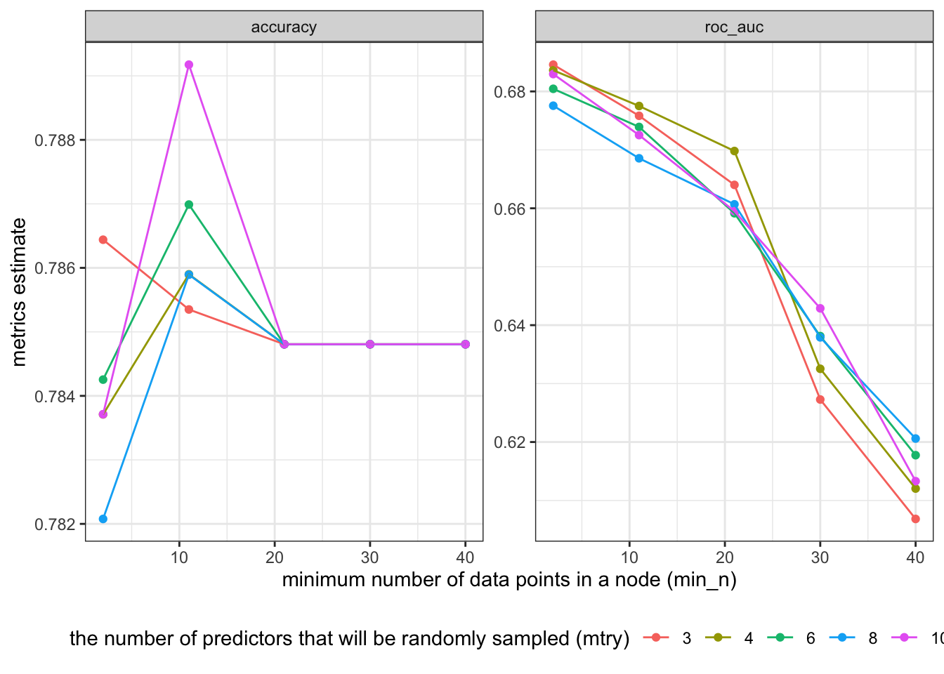

• select hyperparameters and finalize wf

show_best(metric = ) allows to see the top 5 from xg_res %>% collect_metrics()

select_best, select_by_pct_loss, select_by_one_std_err select hyperparameters and corresponding .config to a tibble.

Code

xg_tune_hy <- xg_res %>% 
    select_best(metric = "accuracy")

xg_tune_hy

# A tibble: 1 × 3
   mtry min_n .config              
  <int> <int> <chr>                
1    10    11 Preprocessor1_Model10

finalize model using selected hyperparameters

Code

final_wf <- 
  xg_wf %>% 
  finalize_workflow(xg_tune_hy)

final_wf

══ Workflow ════════════════════════════════════════════════════════════════════
Preprocessor: Recipe
Model: boost_tree()

── Preprocessor ────────────────────────────────────────────────────────────────
3 Recipe Steps

• step_other()
• step_dummy()
• step_zv()

── Model ───────────────────────────────────────────────────────────────────────
Boosted Tree Model Specification (classification)

Main Arguments:
  mtry = 10
  min_n = 11

Computational engine: xgboost 

last_fit model

• use last_fit(split)

Code

final_fit <- final_wf %>% 
    last_fit(chocolate_split)

final_fit

# Resampling results
# Manual resampling 
# A tibble: 1 × 6
  splits             id               .metrics .notes   .predictions .workflow 
  <list>             <chr>            <list>   <list>   <list>       <list>    
1 <split [1831/612]> train/test split <tibble> <tibble> <tibble>     <workflow>

• collect_metrics for overall data

Code

final_fit %>% 
    collect_metrics()

# A tibble: 2 × 4
  .metric  .estimator .estimate .config             
  <chr>    <chr>          <dbl> <chr>               
1 accuracy binary         0.786 Preprocessor1_Model1
2 roc_auc  binary         0.668 Preprocessor1_Model1

metrics are comparable to training data, so not overfiting.

• collect_predictions for test data

Code

final_fit %>% 
    collect_predictions()

# A tibble: 612 × 7
   id               `.pred_< 3` `.pred_>=3`  .row .pred_class rating_bl .config 
   <chr>                  <dbl>       <dbl> <int> <fct>       <fct>     <chr>   
 1 train/test split      0.141        0.859     3 >=3         >=3       Preproc…
 2 train/test split      0.125        0.875    10 >=3         < 3       Preproc…
 3 train/test split      0.0668       0.933    11 >=3         < 3       Preproc…
 4 train/test split      0.156        0.844    17 >=3         >=3       Preproc…
 5 train/test split      0.0668       0.933    24 >=3         >=3       Preproc…
 6 train/test split      0.0668       0.933    25 >=3         >=3       Preproc…
 7 train/test split      0.0711       0.929    32 >=3         >=3       Preproc…
 8 train/test split      0.236        0.764    42 >=3         < 3       Preproc…
 9 train/test split      0.491        0.509    46 >=3         < 3       Preproc…
10 train/test split      0.385        0.615    55 >=3         < 3       Preproc…
# … with 602 more rows
# ℹ Use `print(n = ...)` to see more rows

• roc_auc and roc_curve on test data

calculate roc_auc manually on test data

Code

final_fit %>%
  collect_predictions() %>% 
  roc_auc(truth=rating_bl, `.pred_< 3`)

# A tibble: 1 × 3
  .metric .estimator .estimate
  <chr>   <chr>          <dbl>
1 roc_auc binary         0.668

plot roc_curve

Code

final_fit %>%
  collect_predictions() %>% 
  roc_curve(truth=rating_bl, `.pred_< 3`) %>% 
  autoplot()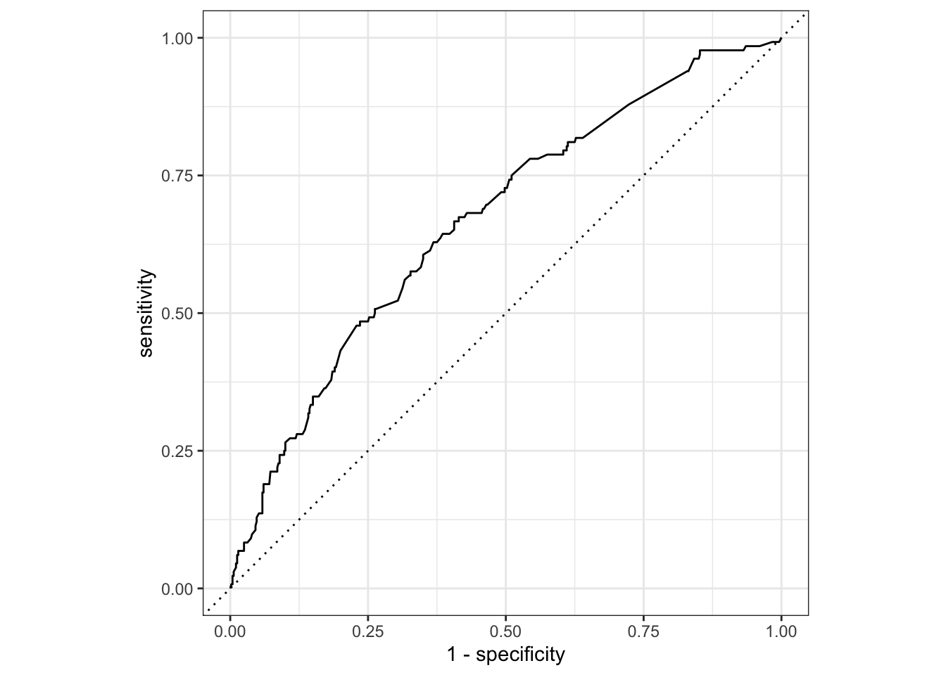

• extract_workflow() to save final_trained_wf

Code

final_trained_wf <- final_fit %>% 
    extract_workflow()

final_trained_wf

══ Workflow [trained] ══════════════════════════════════════════════════════════
Preprocessor: Recipe
Model: boost_tree()

── Preprocessor ────────────────────────────────────────────────────────────────
3 Recipe Steps

• step_other()
• step_dummy()
• step_zv()

── Model ───────────────────────────────────────────────────────────────────────
##### xgb.Booster
raw: 21.7 Kb 
call:
  xgboost::xgb.train(params = list(eta = 0.3, max_depth = 6, gamma = 0, 
    colsample_bytree = 1, colsample_bynode = 0.526315789473684, 
    min_child_weight = 11L, subsample = 1, objective = "binary:logistic"), 
    data = x$data, nrounds = 15, watchlist = x$watchlist, verbose = 0, 
    nthread = 1)
params (as set within xgb.train):
  eta = "0.3", max_depth = "6", gamma = "0", colsample_bytree = "1", colsample_bynode = "0.526315789473684", min_child_weight = "11", subsample = "1", objective = "binary:logistic", nthread = "1", validate_parameters = "TRUE"
xgb.attributes:
  niter
callbacks:
  cb.evaluation.log()
# of features: 19 
niter: 15
nfeatures : 19 
evaluation_log:
    iter training_logloss
       1        0.6020652
       2        0.5525599
---                      
      14        0.4693209
      15        0.4688216

• extract_* information from final_trained_wf

  • extract_fit_engine() is engine-specific model

Code

final_trained_wf %>%
  extract_fit_engine()

##### xgb.Booster
raw: 21.7 Kb 
call:
  xgboost::xgb.train(params = list(eta = 0.3, max_depth = 6, gamma = 0, 
    colsample_bytree = 1, colsample_bynode = 0.526315789473684, 
    min_child_weight = 11L, subsample = 1, objective = "binary:logistic"), 
    data = x$data, nrounds = 15, watchlist = x$watchlist, verbose = 0, 
    nthread = 1)
params (as set within xgb.train):
  eta = "0.3", max_depth = "6", gamma = "0", colsample_bytree = "1", colsample_bynode = "0.526315789473684", min_child_weight = "11", subsample = "1", objective = "binary:logistic", nthread = "1", validate_parameters = "TRUE"
xgb.attributes:
  niter
callbacks:
  cb.evaluation.log()
# of features: 19 
niter: 15
nfeatures : 19 
evaluation_log:
    iter training_logloss
       1        0.6020652
       2        0.5525599
---                      
      14        0.4693209
      15        0.4688216

• extract_fit_parsnip() is parsnip model object

Code

final_trained_wf %>%
  extract_fit_parsnip()

parsnip model object

##### xgb.Booster
raw: 21.7 Kb 
call:
  xgboost::xgb.train(params = list(eta = 0.3, max_depth = 6, gamma = 0, 
    colsample_bytree = 1, colsample_bynode = 0.526315789473684, 
    min_child_weight = 11L, subsample = 1, objective = "binary:logistic"), 
    data = x$data, nrounds = 15, watchlist = x$watchlist, verbose = 0, 
    nthread = 1)
params (as set within xgb.train):
  eta = "0.3", max_depth = "6", gamma = "0", colsample_bytree = "1", colsample_bynode = "0.526315789473684", min_child_weight = "11", subsample = "1", objective = "binary:logistic", nthread = "1", validate_parameters = "TRUE"
xgb.attributes:
  niter
callbacks:
  cb.evaluation.log()
# of features: 19 
niter: 15
nfeatures : 19 
evaluation_log:
    iter training_logloss
       1        0.6020652
       2        0.5525599
---                      
      14        0.4693209
      15        0.4688216

• extract_recipe or extract_preprocessing to get recipe/preprocessing

Code

final_trained_wf %>% extract_preprocessor()

Recipe

Inputs:

      role #variables
   outcome          1
 predictor         16

Operations:

Collapsing factor levels for company_manufacturer
Dummy variables from all_nominal_predictors()
Zero variance filter on all_predictors()

feature importance

• vip() plot top 10
• vi_model() return tibble

Code

final_trained_wf %>%
  extract_fit_parsnip() %>% 
  vip()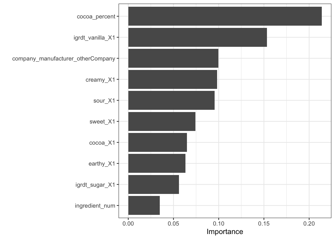

Final notes

• I convert numeric rating to categorical rating using threshold because, based on the exploratory analysis, the rating values are not continuous.
• The boost_tree did not produce good estimate for the data.
  • Other models, like rand_forest(), logistic_reg and svm_linear are worth to try.
  • Tuning other hyperparameters tree_depth, learning_rate and trees are worth to try. I don’t know which tune-able hyperparameter corresponds to regularization gamma.
• Julia Silge posted a screencast and blog of using rand_forest() and svm_linear training rating as linear model on the same dataset.