TidyTuesday: predict ultra race time

tidyTuesday

tidymodels

Author

Chun Su

Published

November 2, 2021

Load required libraries

Code

library(tidyverse)
library(tidymodels)
library(lubridate)

data skim

Data README is available at here.

Code

ultra_rankings <- tuesdata$ultra_rankings
race <- tuesdata$race

ultra_join <-
    ultra_rankings %>% 
    left_join(race, by="race_year_id")

Code

skimr::skim(ultra_join)

Data summary
Name	ultra_join
Number of rows	137803
Number of columns	20
_______________________
Column type frequency:
character	9
Date	1
difftime	1
numeric	9
________________________
Group variables	None

Variable type: character

skim_variable	n_missing	complete_rate	min	max	n_unique
runner	0	1.00	3	52	73629
time	17791	0.87	8	11	72840
gender	30	1.00	1	1	2
nationality	0	1.00	3	3	133
event	0	1.00	4	57	435
race	0	1.00	3	63	371
city	15599	0.89	2	30	308
country	77	1.00	4	17	60
participation	0	1.00	4	5	4

Variable type: Date

skim_variable	n_missing	complete_rate	min	max	median	n_unique
date	0	1	2012-01-14	2021-09-03	2017-10-13	711

Variable type: difftime

skim_variable	n_missing	complete_rate	min	max	median	n_unique
start_time	0	1	0 secs	82800 secs	05:00:00	39

Variable type: numeric

skim_variable	n_missing	complete_rate	mean	sd	p0	p25	p50	p75	p100	hist
race_year_id	0	1.00	26678.70	20156.18	2320	8670.0	21795.0	40621	72496.0	▇▃▃▂▂
rank	17791	0.87	253.56	390.80	1	31.0	87.0	235	1962.0	▇▁▁▁▁
age	0	1.00	46.25	10.11	0	40.0	46.0	53	133.0	▁▇▂▁▁
time_in_seconds	17791	0.87	122358.26	37234.38	3600	96566.0	114167.0	148020	296806.0	▁▇▆▁▁
distance	0	1.00	154.08	39.22	0	160.9	162.6	168	179.1	▁▁▁▁▇
elevation_gain	0	1.00	6473.94	3293.50	0	3910.0	6640.0	9618	14430.0	▅▆▆▇▁
elevation_loss	0	1.00	-6512.20	3305.73	-14440	-9618.0	-6810.0	-3950	0.0	▁▇▆▅▅
aid_stations	0	1.00	9.58	7.56	0	0.0	12.0	16	56.0	▇▇▁▁▁
participants	0	1.00	510.75	881.25	0	0.0	65.0	400	2900.0	▇▁▁▁▁

EDA

We want to estimate the time (time_in_seconds) for runner to finish based on the features.

the effect of gender and age

Code

ultra_join %>% 
    filter(!is.na(time_in_seconds)) %>% 
    filter(!is.na(gender)) %>% 
    filter(age > 10, age < 100) %>% 
    mutate(age_decade = 5* (age %/% 5)) %>% 
    select(time_in_seconds, gender, age, age_decade) %>% 
    group_by(age_decade, gender) %>% 
    summarise(
        time_in_seconds_sd = sd(time_in_seconds),
         time_in_seconds = mean(time_in_seconds)
    ) %>% 
    ggplot(aes(x = age_decade, color=gender, group=gender)) +
    geom_point(aes(y=time_in_seconds)) +
    geom_line(aes(y=time_in_seconds)) +
    geom_errorbar(aes(ymin=time_in_seconds - time_in_seconds_sd, ymax=time_in_seconds + time_in_seconds_sd), width=0.2, alpha=0.7) +
    scale_color_viridis_d() +
    labs(x = "age", y = "time (second)") +
    scale_y_continuous(labels = scales::label_comma())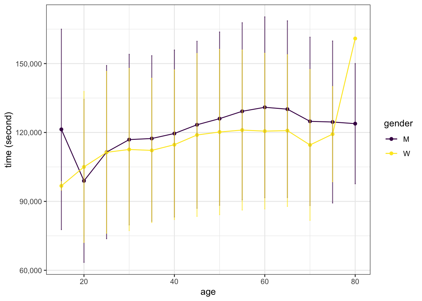

the effect of nationality, age, gender

Code

ultra_join %>% 
    mutate(nationality = fct_lump(nationality, prop=0.05)) %>% 
    count(nationality, sort=TRUE)

# A tibble: 4 × 2
  nationality     n
  <fct>       <int>
1 Other       50563
2 USA         47259
3 FRA         28905
4 GBR         11076

Code

ultra_join %>% 
    filter(!is.na(time_in_seconds)) %>% 
    filter(!is.na(gender)) %>% 
    filter(age > 10, age < 100) %>% 
    mutate(nationality = fct_lump(nationality, prop=0.05)) %>% 
    ggplot(aes(x = age, fill=nationality), group=nationality) +
    facet_wrap(vars(gender)) +
    geom_bar(stat="density", alpha=0.5)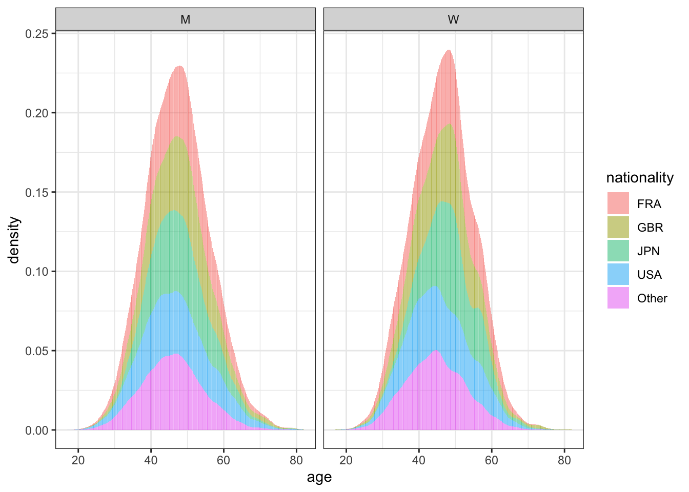

nationality

Code

ultra_join %>% 
    filter(!is.na(time_in_seconds)) %>% 
    filter(!is.na(gender)) %>% 
    filter(age > 10, age < 100) %>% 
    mutate(nationality = fct_lump(nationality, prop=0.05)) %>% 
    ggplot(aes(x=fct_reorder(nationality, time_in_seconds), y=time_in_seconds, fill=nationality)) +
    geom_boxplot() +
    scale_fill_viridis_d() +
    labs(x="runner's nationality", fill=NULL, y="time (second)") +
    scale_y_continuous(labels = scales::label_comma())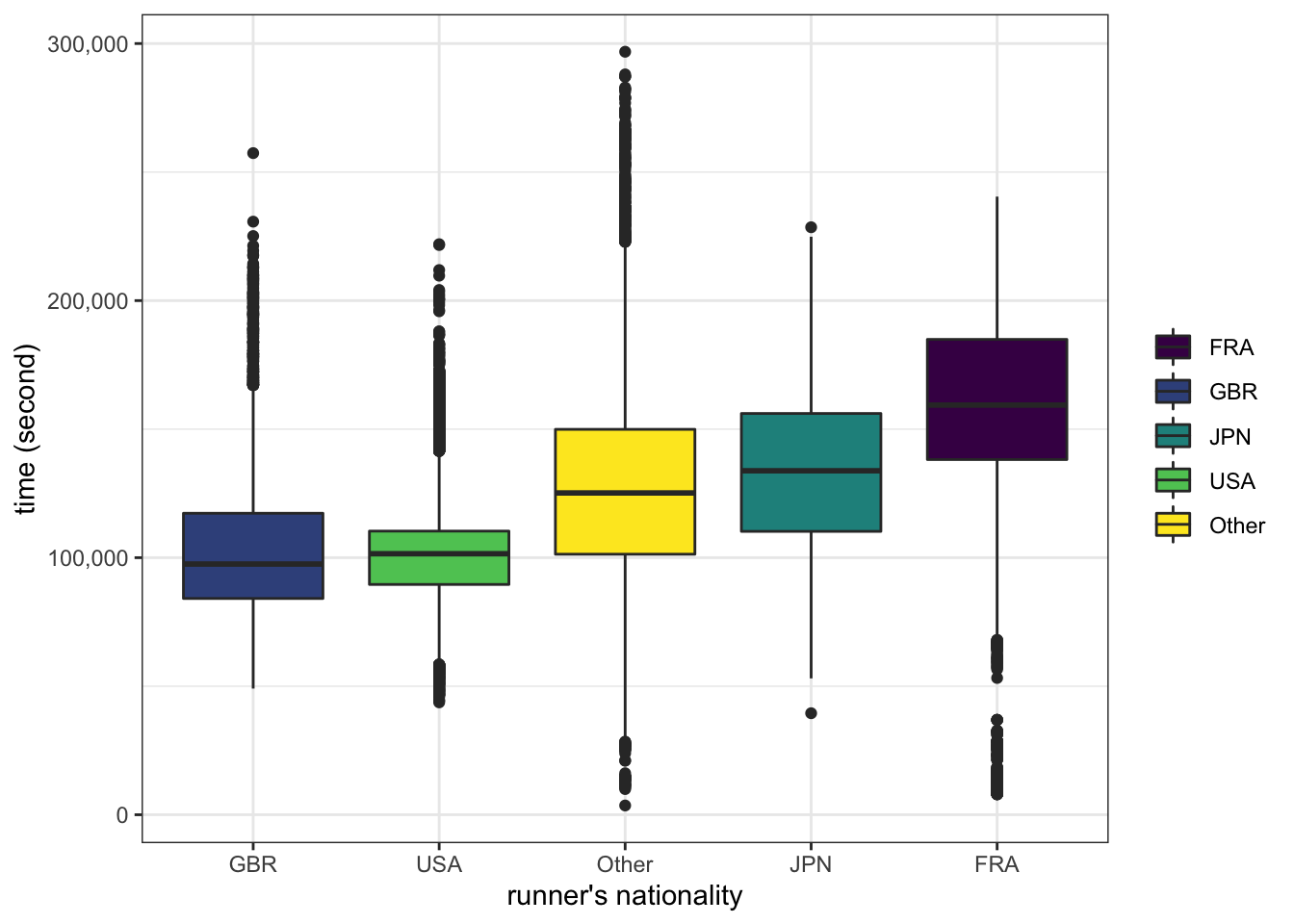

effect of distance

Code

ultra_join %>% 
    filter(!is.na(time_in_seconds)) %>% 
    filter(distance >= 150) %>% 
    ggplot(aes(x=distance, y=time_in_seconds)) +
    geom_point(alpha=0.1, size=1) +
    geom_smooth() +
    labs(y="time (second)") +
    scale_y_continuous(labels = scales::label_comma())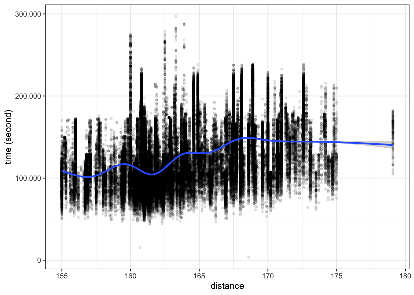

effect of elevation

Code

ultra_join %>% 
    filter(!is.na(time_in_seconds)) %>% 
    filter(distance >= 150) %>% 
    mutate(elevation = ifelse(
        elevation_gain > abs(elevation_loss), elevation_gain,  abs(elevation_loss)
        )) %>% 
    ggplot(aes(x=elevation , y=time_in_seconds)) +
    geom_point(alpha=0.1, size=1) +
    geom_smooth() +
    labs(y="time (second)") +
    scale_y_continuous(labels = scales::label_comma())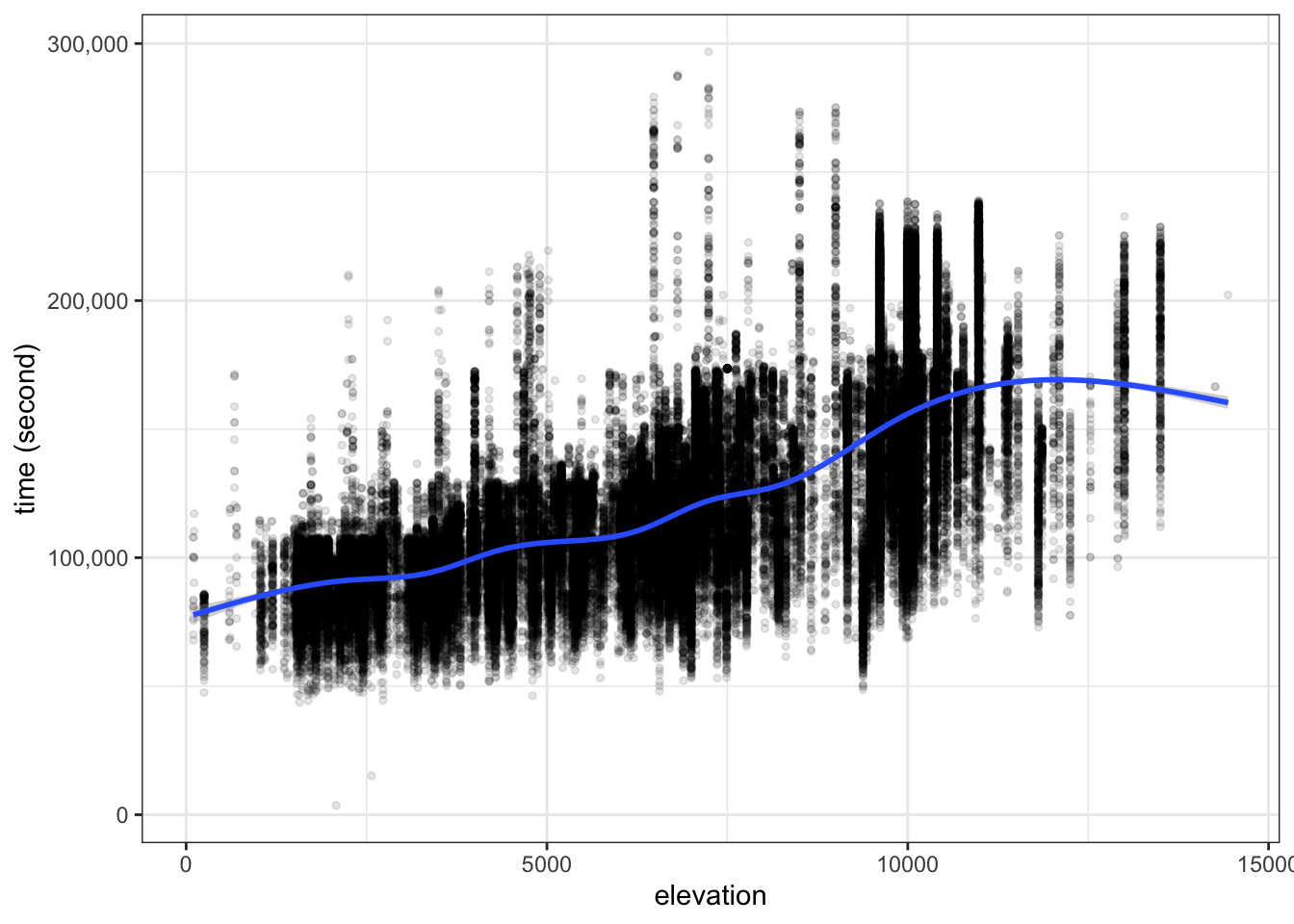

effect of date

The year of the race

Code

ultra_join %>% 
    filter(!is.na(time_in_seconds)) %>% 
    mutate(
        race_year=lubridate::year(date), 
        race_month=lubridate::month(date)
    ) %>% 
    group_by(race_year) %>% 
    summarise(
        time_in_seconds_sd=mean(time_in_seconds),
        time_in_seconds=mean(time_in_seconds)
    ) %>% 
    ungroup() %>% 
    ggplot(aes(x=race_year, y=time_in_seconds)) +
    geom_point() +
    geom_line() +
    geom_errorbar(aes(ymin=time_in_seconds - time_in_seconds_sd, ymax=time_in_seconds + time_in_seconds_sd), alpha=0.5)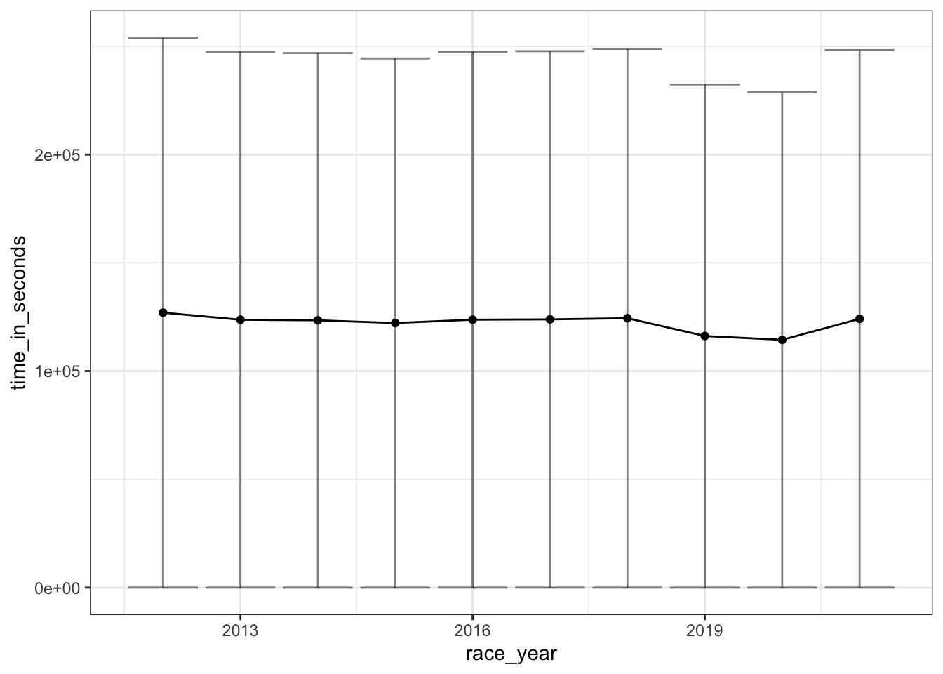

The month of race can be the proxy to estimate the season when race was hosted. However, here I did not take the geographic information (hemisphere) into consideration.

Code

ultra_join %>% 
    filter(!is.na(time_in_seconds)) %>% 
    mutate(
        race_year=lubridate::year(date), 
        race_month=lubridate::month(date)
    ) %>% 
    group_by(race_month) %>% 
    summarise(
        time_in_seconds_sd=mean(time_in_seconds),
        time_in_seconds=mean(time_in_seconds)
    ) %>% 
    ungroup() %>% 
    ggplot(aes(x=race_month, y=time_in_seconds)) +
    geom_point() +
    geom_line() +
    geom_errorbar(aes(ymin=time_in_seconds - time_in_seconds_sd, ymax=time_in_seconds + time_in_seconds_sd), alpha=0.5)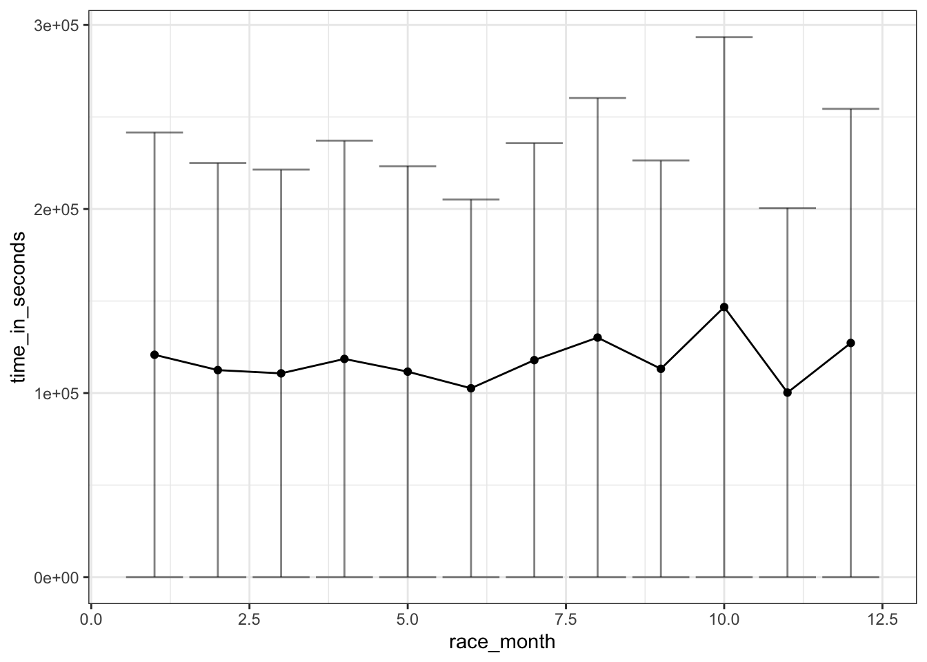

learning models

Here I will perform two distinct models – linear regression and random forest to predict the race time using runner’s gender, age, nationality, elevation and distance of race.

data budget

inistal split to train and test

Code

ultra_df <- ultra_join %>% 
  filter(!is.na(time_in_seconds)) %>% 
  filter(!is.na(gender)) %>% 
  filter(age > 10, age < 100) %>% 
  filter(distance >= 150) %>% 
  mutate(elevation = ifelse(
        elevation_gain > abs(elevation_loss), 
        elevation_gain,
        abs(elevation_loss)
        )
  ) %>% 
  select(time_in_seconds, age, gender, nationality, distance, elevation)

set.seed(2021)
ultra_split <- initial_split(ultra_df, strata = time_in_seconds)
ultra_train <- training(ultra_split)
ultra_test <- testing(ultra_split)

create resamples for cross validation

Code

set.seed(124)
ultra_folds <- vfold_cv(ultra_train, v=10)

recipes for feature engineer

Code

ultra_rec <- recipe(time_in_seconds ~., data = ultra_train) %>% 
  step_other(nationality) %>% 
  step_normalize(all_numeric_predictors()) %>% 
  step_string2factor(all_nominal_predictors()) %>% 
  # step_dummy(all_nominal_predictors()) %>% 
  I()

# want to test whether dummy variables affect the model behave
ind_rec <- ultra_rec %>% 
  step_dummy(all_nominal_predictors())

fit linear model

specify models

Code

lm_spec <- linear_reg() %>% 
  set_engine('lm') %>% 
  set_mode('regression')

Does linear model need dummy variable? Using workflow_set to test

Code

lm_wf <- workflow_set(
  preproc = list("nodummy"=ultra_rec, "dummy"=ind_rec),
  models = list(lm_spec)
)

lm_rs <- workflow_map(
  lm_wf, 'fit_resamples', resamples=ultra_folds
  )

lm_rs %>% collect_metrics()

# A tibble: 4 × 9
  wflow_id           .config preproc model .metric .esti…¹    mean     n std_err
  <chr>              <chr>   <chr>   <chr> <chr>   <chr>     <dbl> <int>   <dbl>
1 nodummy_linear_reg Prepro… AsIs    line… rmse    standa… 2.39e+4    10 6.94e+1
2 nodummy_linear_reg Prepro… AsIs    line… rsq     standa… 5.66e-1    10 2.73e-3
3 dummy_linear_reg   Prepro… AsIs    line… rmse    standa… 2.39e+4    10 6.94e+1
4 dummy_linear_reg   Prepro… AsIs    line… rsq     standa… 5.66e-1    10 2.73e-3
# … with abbreviated variable name ¹.estimator

Based on the r-square value, the linear model with age, distance, elevation, gender and nationality explained ~57% variance of time_in_seconds.

Using dummy variable or not does not change the metrics. In fact, the number of coefficients will be exactly same no matter whether using dummy or not. Below shows coefficients of linear regression by fitting the “nodummy_linear_reg” workflow to the training data.

Code

lm_coef <- lm_rs %>% 
  extract_workflow('nodummy_linear_reg') %>% 
  fit(ultra_train) %>% 
  tidy()

lm_coef

# A tibble: 9 × 5
  term             estimate std.error statistic   p.value
  <chr>               <dbl>     <dbl>     <dbl>     <dbl>
1 (Intercept)       142711.     217.      658.  0        
2 age                 4220.      83.3      50.6 0        
3 genderW             6315.     236.       26.8 1.82e-157
4 nationalityGBR    -25432.     389.      -65.3 0        
5 nationalityJPN    -20211.     406.      -49.8 0        
6 nationalityUSA    -30025.     302.      -99.6 0        
7 nationalityother  -19682.     254.      -77.6 0        
8 distance            2630.      99.2      26.5 2.65e-154
9 elevation          17421.     117.      149.  0

Code

lm_coef %>% 
  filter(term!="(Intercept)") %>% 
  ggplot(aes(x = estimate, y = fct_reorder(term, estimate))) +
  geom_col(aes(fill=(estimate < 0)), alpha = 0.5) +
  geom_errorbar(aes(xmin=estimate - std.error, xmax = estimate + std.error), width=0.5) +
  theme(legend.position = 'none') +
  labs(fill=NULL, y = NULL)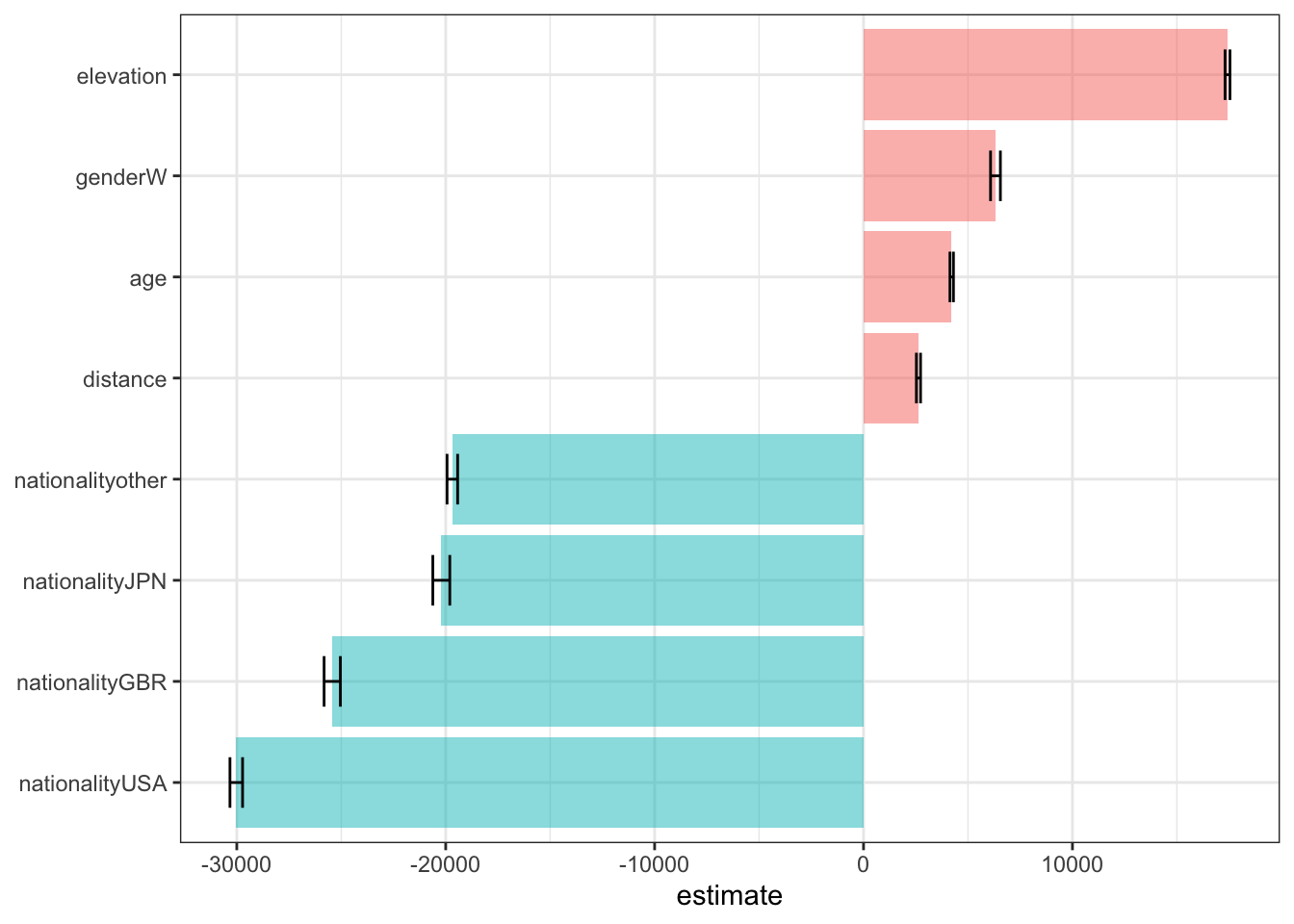

Elevation, being a women (compare to being a men), age and distance positively affect race time, while racers from JPN/GBR/USA/other (compare to racers from FRA) finish the race in shorter time.

fit random forest model using workflow

Using random forest as model to get Resampling results

Code

rf_spec <- rand_forest() %>% 
  set_engine('ranger') %>% 
  set_mode('regression')

rf_wf <- workflow() %>% 
  add_model(rf_spec) %>% 
  add_recipe(ultra_rec)

# resample evaluate 
rf_rs  <- rf_wf %>% 
  fit_resamples(
    resamples = ultra_folds
  )

Code

rf_rs  %>% 
  collect_metrics()

# A tibble: 2 × 6
  .metric .estimator      mean     n  std_err .config             
  <chr>   <chr>          <dbl> <int>    <dbl> <chr>               
1 rmse    standard   18535.       10 57.2     Preprocessor1_Model1
2 rsq     standard       0.738    10  0.00219 Preprocessor1_Model1

Compared to linear model shown above, random forest with same predictors can explain more variance of Y (74% vs. 56%) and show smaller rmse (1.8e4 vs. 2.4e4).

Code

bind_rows(
  rf_rs  %>% 
    collect_metrics() %>% 
    select(.metric, mean, std_err) %>% 
    mutate(model = "random forest"),
  lm_rs  %>% 
    collect_metrics() %>% 
    filter(wflow_id == 'nodummy_linear_reg') %>% 
    select(.metric, mean, std_err) %>% 
    mutate(model = "linear reg")
) %>% 
  ggplot(aes(x = model, y = mean)) +
  facet_wrap(vars(.metric), scales = 'free') +
  geom_point() +
  geom_errorbar(aes(ymin=mean - std_err, ymax=mean + std_err), width=0)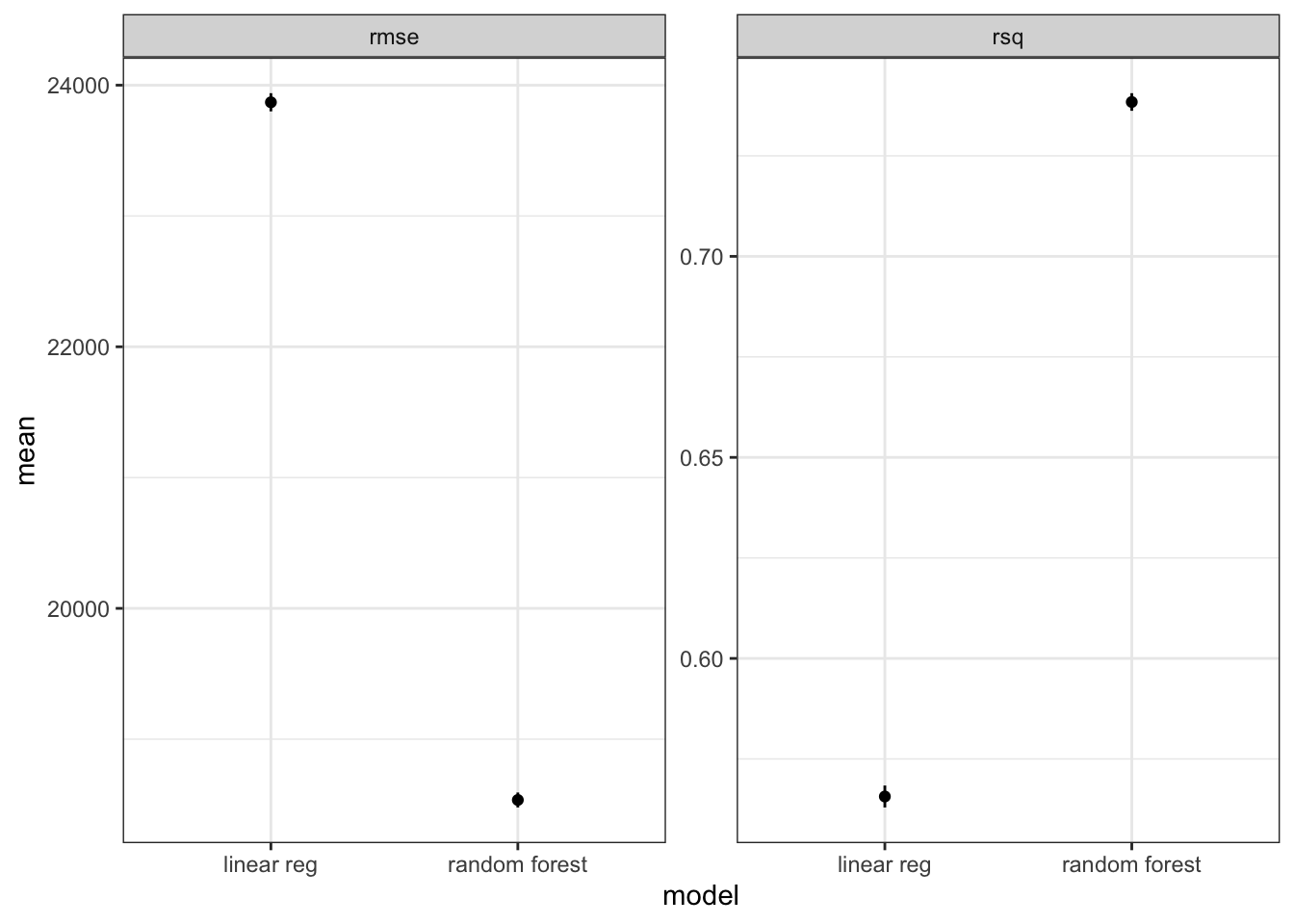

Notes: above plot can also be done by autoplot if we perform the comparison between linear regression and random forest models using workflow_set.

`last_fit` test data using random forest result

Code

rf_final_rs <- rf_wf %>% 
  last_fit(ultra_split)

Code

rf_final_rs %>% 
  collect_metrics()

# A tibble: 2 × 4
  .metric .estimator .estimate .config             
  <chr>   <chr>          <dbl> <chr>               
1 rmse    standard   18558.    Preprocessor1_Model1
2 rsq     standard       0.737 Preprocessor1_Model1

Different from fit_resample results, these metrics are calculated on the test data. The value is very close to the values done on training data (resample data), thus the model is not over-fitted.

Code

final_wf <- rf_final_rs %>% 
  extract_workflow()

final_wf

══ Workflow [trained] ══════════════════════════════════════════════════════════
Preprocessor: Recipe
Model: rand_forest()

── Preprocessor ────────────────────────────────────────────────────────────────
3 Recipe Steps

• step_other()
• step_normalize()
• step_string2factor()

── Model ───────────────────────────────────────────────────────────────────────
Ranger result

Call:
 ranger::ranger(x = maybe_data_frame(x), y = y, num.threads = 1,      verbose = FALSE, seed = sample.int(10^5, 1)) 

Type:                             Regression 
Number of trees:                  500 
Sample size:                      83042 
Number of independent variables:  5 
Mtry:                             2 
Target node size:                 5 
Variable importance mode:         none 
Splitrule:                        variance 
OOB prediction error (MSE):       342750489 
R squared (OOB):                  0.7386915

The above trained workflow from last_fit can be saved in .rda for future prediction

Code

# using final_wf for prediction
final_wf %>% 
  predict(new_data = ultra_train %>% dplyr::slice(1))

# A tibble: 1 × 1
    .pred
    <dbl>
1 108741.

what techniques i learned

deal with high-levels nominal features (fct_lump and step_other) in EDA and modeling
workflow_set and map_workflow to create multiple workflows for model and/or recipes comparison.
fit_resample for cross-validation. The metrics collected from cross-validation results are used for workflow comparison.
last_fit model and save trained workflow for future use

data skim

EDA

the effect of gender and age

the effect of nationality, age, gender

effect of distance

effect of elevation

effect of date

learning models

data budget

recipes for feature engineer

fit linear model

fit random forest model using workflow

last_fit test data using random forest result

what techniques i learned

`last_fit` test data using random forest result