I have been performing survival analysis for a while. Although I can create standard survival curves and summarize hypothesis testing tables, I have never really UNDERSTOOD it until recently. In this post, I will share some of my study notes to dive into the concepts, assumptions, deduction and result interpretations on survival analysis, using the Cancer Genome Atlas (TCGA) clinical data 1 as example.
Basic concepts
censoring
Censoring is a condition in which the value of a measurement or observation is only partially known 2. In clinical trial, a sample is labeled censored when information on time to event is unavailable due to the loss to follow-up or non-occurrence of outcome event before the trial end. The event can be death or disease relapse.
clinical outcome endpoint
Overall survival (OS)
disease-specific survival (DSS)
disease-free interval (DFI)
progression-free interval (PFI)
Compared to DFI and PFI, OS or DSS demands longer follow-up time because patients generally develop disease recurrence or progression before dying of their disease.
Selection of a specific survival endpoint also depends on the study goal.
A clinical trial testing the effect of a drug’s ability to delay or prevent cancer progression would use PFI as the most appropriate endpoint.
In TCGA clinical data, the short-term clinical follow-up intervals favor outcome analyses in more aggressive cancer types, which are likely to observe events within a couple of years. Studies with less aggressive cancer types, in which patients relapse only after many years or even decades, may not observe enough events during their follow-up intervals to support reliable outcome determinations 3.
survival time (T) vs. censoring time (C)
survival time: the true time at which event occurs: occur before trial ends (\(T < period limit\)), occur after trial ends (\(T > period limit\))
censoring time: time at which drop out (\(C < period limit\)) or study ends (\(C = period limit\))
observed pair (Y, sigma)
random variable: \(Y = min(T, C)\)
status indicator: \(\sigma\) = 1 or 0
No event - sigma = 0: Y = C; drop out (\(T > C\), \(\sigma\) = 0) or survived beyond (\(T > C\), \(\sigma\)=0)
With event - sigma = 1: Y = T; event happened (T ≤ C, \(\sigma\) = 1)
censoring types
right censoring: T ≥ Y (expected Y ≤ period limit, with event (sigma=1) is defined as \(T < limit\)). This is the most common one.
left censoring: T ≤ Y (expected Y ≥ period limit; with event (sigma=1) is defined as \(T > limit\))
internal censoring: we do not know T value ( limit 0 ≤ expected Y ≤ limit 1; with event (sigma=1) is defined as T within (limit 0, limit 1))
survival analysis assumption
censoring mechanism is independent: conditional on the features, the event time T is independent of the censoring time C
The examples that violated this assumption can be a number of patients drop out (C) of a cancer study early because they are very sick (T). Or males who are very sick (T) are more likely to drop out (C) of the study than females who are very sick.
Kaplan-Meier survival curve
S(t) = Pr(T > t)
\(S(t) = Pr(T > t)\): the probability of surviving past time t. The larger the value of S(t), the less likely that the patient will die before time t.
However, due to the censoring in the data, we do not always know T. Instead we can only read observed pair \((Y,\sigma)\) in which Y = min(T,C).
K-M estimator
K-M estimator is a product limit estimator to estimate S(t) using \((Y, \sigma)\).
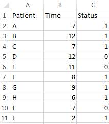
sort all censored samples (\(\sigma=0\)) based on their T (here Y = T), and the new rank become \(i\), and the survival time at each rank is \(t_i\).
count the number of samples not dead \(n_i\) at \(t_i\). This number can be any sample (no matter censored or not) with \(Y > t_i\). it is also called “samples at risk”.
count the number of samples died \(d_i\) at time point \(t_i\).
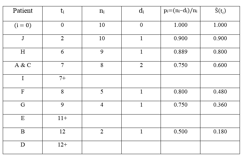
to estimate S(t), calculate surviving proportion (\(p_i\)) at each censored time (\(t_i\)).
\[p_i = (n_i - d_i)/n_i\]
The \(S\hat(t{i})\) is the product of all censored \(p_i\) before \(t_i\).
\[S\hat(t_i) = \prod_{1}^{i} p_i\].
Xu wrote make a “AHA” example to show how \(S\hat(t_i)\) was calculated 4.
The process to calculate K-M estimator:
Because of product limit estimator, the K-M survival curve is step-like, in which x axis represents \(t_i\) and y represents \(S\hat(t_i)\).
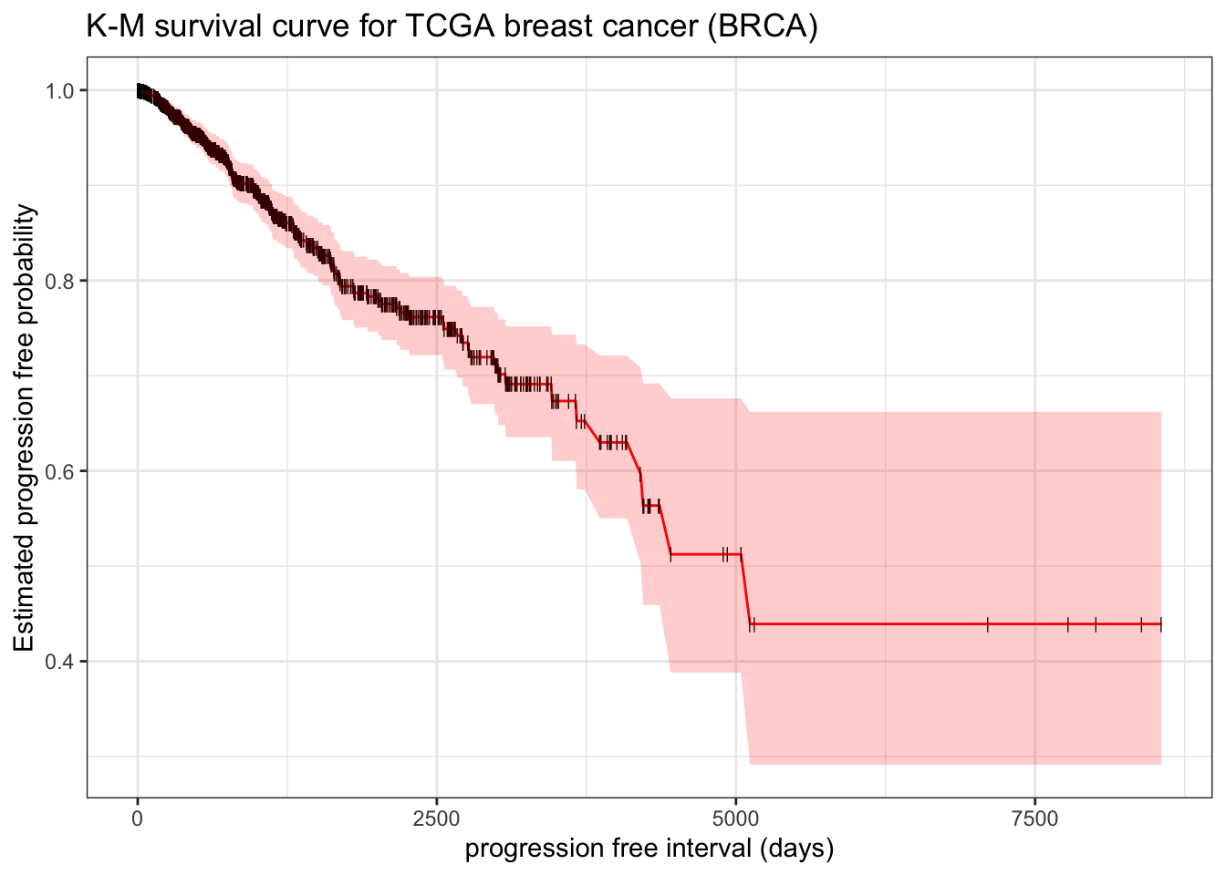
example: make a survival curve in TCGA breast cancer survfit
Here we use progression free interval (PFI) as outcome endpoint.
library(survival)library(tidyverse)theme_set(theme_bw())# clinical datatcga_cdr <- openxlsx::read.xlsx("https://www.cell.com/cms/10.1016/j.cell.2018.02.052/attachment/bbf46a06-1fb0-417a-a259-fd47591180e4/mmc1.xlsx") |>as_tibble() |> janitor::clean_names() |>filter(type=="BRCA")fit.surv <-survfit(Surv(pfi_time, pfi) ~1, data = tcga_cdr) # be aware pfi must be numeric, otherwise it will trigger multi-state modelbroom::tidy(fit.surv)
It reports result like above Xu’s manual calculation table. estimate represent the \(S(t)\). Thus to manually plot K-M survival curve,
broom::tidy(fit.surv) |>ggplot(aes(x = time, y = estimate)) +geom_line(color ="red") +geom_point(shape="|", size=2) +geom_ribbon(aes(ymax = conf.high, ymin = conf.low), alpha=0.2, fill="red") +# add confident interval for estimated S(t)labs(x ="progression free interval (days)", y ="Estimated progression free probability") +ggtitle("K-M survival curve for TCGA breast cancer (BRCA)")
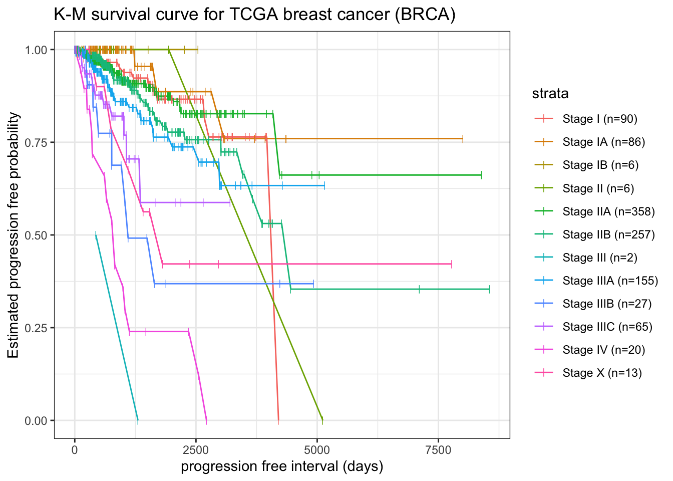
To stratify survival curve by pathologic stage (ajcc_pathologic_tumor_stage)
fit.surv2 <-survfit(Surv(pfi_time, pfi) ~ ajcc_pathologic_tumor_stage, data = tcga_cdr)broom::tidy(fit.surv2) |>left_join( broom::tidy(fit.surv2) |>group_by(strata) |> dplyr::slice(which.min(time)) |>select(n = n.risk, strata) ) |>mutate(strata =str_replace(strata, ".*=", "")) |>filter(!grepl("\\[", strata)) |>mutate(strata = glue::glue("{strata} (n={n})")) |>ggplot(aes(x = time, y = estimate, group = strata)) +geom_line(aes(color = strata)) +geom_point(aes(color = strata), shape="|", size=2) +labs(x ="progression free interval (days)", y ="Estimated progression free probability") +ggtitle("K-M survival curve for TCGA breast cancer (BRCA)")
Note: here for stage III, t0 is not start with day0 and 1 out of 2 risk samples with event, thus S(t) start with 0.5 instead of 1.
Beside manually plotting survival curve using ggplot, autoplot from R package {ggfortify} can automatically plot beautiful curves. Refer to ggfortify autoplot tutorial to know more.
In addition, R package {survminer} also provide functions for facilitating survival analysis and visualization (ggsurvplot). The advantage of use this package over ggplot or autoplot is that it can automatically add risk table under plot.
log-rank test
The log-rank test is a nonparametric hypothesis test to test whether there is difference between two independent groups.
Chi-squared test like log-rank statistics.
It can be calculated pretty much in the same way as chi-square test \(\chi^2 = \sum((O_i - E_i)^2/E_i)\)
expected sample number to be dead in group A \(E_{Ai}\) at time point \(t_i\).
As noted, there are several variations of the log rank statistic 5. Some statistical computing packages use the following test statistic for the log rank test to compare two independent groups:
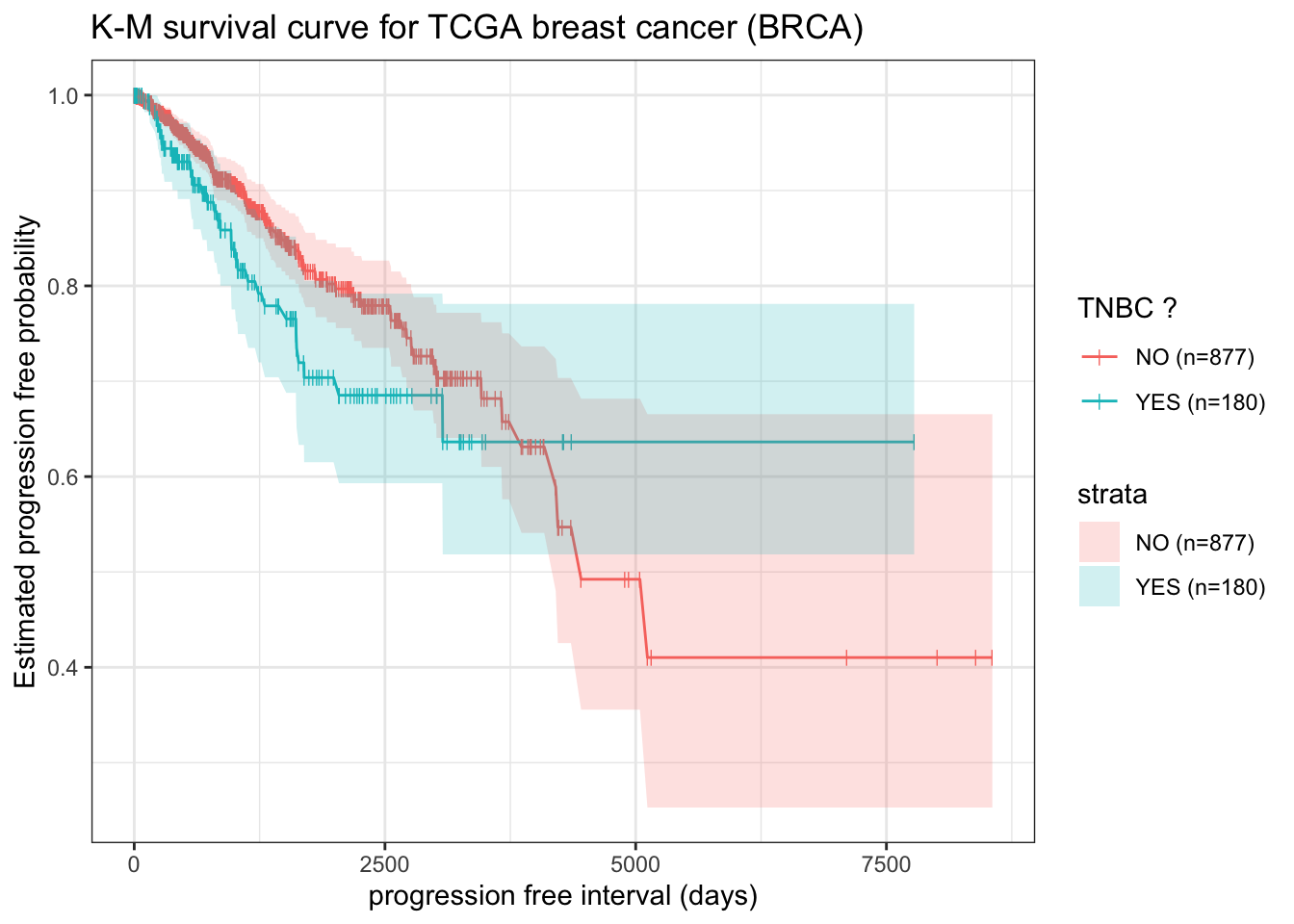
example: survdiff to test TNBC and non-TNBC difference
The triple-negative breast cancer (TNBC) is one type of breast cancers without expression of estrogen receptor (ER), progesterone receptor (PR) or HER2 amplification. The Patients with TNBC are presented with worse overall prognoses and lack of effective targeted treatment options 6. Lehmann et al used a two-component Gaussian mixture model (R package {optim}) to estimate the posterior probability of negative expression status of ER, PR and HER2, and identified TNBC patients from TCGA gene expression data 7. Here we will combine above data.frame tcga_cdr with TNBC annotation from Lehmann et al 2016 8 and perform log.rank test (survdiff) to estimate whether TNBC patients have worse overall prognoses as stated.
# A tibble: 2 × 4
  tnbc      N   obs   exp
  <chr> <dbl> <dbl> <dbl>
1 NO      877   108 116.
2 YES     180    33  24.7
broom::tidy(fit.surv3) reports chi-square like table with summary statistics of total sample (N), observed sample number with event (obs), expected sample number with event (exp) for each group.
broom::tidy(fit.surv3)
# A tibble: 2 × 4
  tnbc      N   obs   exp
  <chr> <dbl> <dbl> <dbl>
1 NO      877   108 116.
2 YES     180    33  24.7
broom::tidy(fit.surv3) reports summary statistics on chi-square (estimate), degree of freedom (df) and p-value (p.value)
In our case, using alpha = 0.05 as cutoff, log.rank test indicates TNBC shows no significant difference from non-TNBC patients on probability of tumor progression.
Since the coxph test is a more complicated concept and requires additional prerequisite statistics terms, it will be discussed in detail at part 2. Stay tuned!
Kalecky, K., Modisette, R., Pena, S. et al. Integrative analysis of breast cancer profiles in TCGA by TNBC subgrouping reveals novel microRNA-specific clusters, including miR-17-92a, distinguishing basal-like 1 and basal-like 2 TNBC subtypes. BMC Cancer 20, 141 (2020). https://doi.org/10.1186/s12885-020-6600-6↩︎
Lehmann BD, Jovanović B, Chen X, Estrada MV, Johnson KN, Shyr Y, et al. (2016) Refinement of Triple-Negative Breast Cancer Molecular Subtypes: Implications for Neoadjuvant Chemotherapy Selection. PLoS ONE 11(6): e0157368. https://doi.org/10.1371/journal.pone.0157368↩︎
Lehmann BD, Jovanović B, Chen X, Estrada MV, Johnson KN, Shyr Y, et al. (2016) Refinement of Triple-Negative Breast Cancer Molecular Subtypes: Implications for Neoadjuvant Chemotherapy Selection. PLoS ONE 11(6): e0157368. https://doi.org/10.1371/journal.pone.0157368↩︎