Interpreting the coefficients of Generalized Linear Model

GLM

tidymodels

Author

Chun Su

Published

February 28, 2022

Linear model is the most popular model used in various of fields, due to its simple execution and interpretation. It can be not only used to predict like all other machine learning models. but also widely used for statistical inference due to its simplicity.

Generalized Linear Model (GLM), as named indicated, is generalized from linear regression model, and extends linear model default assumptions to include outcome variables following exponential family distribution. It used link function to transform the outcome so that the transformed Y can be represented by linear combination of predictors. Due to this transformation, it makes coefficients interpretation a little confusing. In this blog, I will use four classical examples (Boston, Default, BrainCancer, and Bikeshare from ISLR2 package) to illustrate how to interpret the coefficients of GLM from tidymodels fit tidy outcome in R.

Code

library(ISLR2)
library(tidyverse)
library(tidymodels)

Linear regression

Modeling linear regression in R is simple. The following example used dis (weighted mean of distances to five Boston employment centers) as single predictor to predict medv (median value of house in $1000s) in Boston.

Code

data(Boston)
lm_m1 <- lm(medv ~ dis, data = Boston)
summary(lm_m1)


Call:
lm(formula = medv ~ dis, data = Boston)

Residuals:
    Min      1Q  Median      3Q     Max 
-15.016  -5.556  -1.865   2.288  30.377 

Coefficients:
            Estimate Std. Error t value Pr(>|t|)    
(Intercept)  18.3901     0.8174  22.499  < 2e-16 ***
dis           1.0916     0.1884   5.795 1.21e-08 ***
---
Signif. codes:  0 '***' 0.001 '**' 0.01 '*' 0.05 '.' 0.1 ' ' 1

Residual standard error: 8.914 on 504 degrees of freedom
Multiple R-squared:  0.06246,   Adjusted R-squared:  0.0606 
F-statistic: 33.58 on 1 and 504 DF,  p-value: 1.207e-08

Based on coefficients summary, dis is significantly (p-value = 1.21e-08) positively correlated with medv. With 1 unit increase in term of distances to Boston employment centers, the median value of house increase $1091.6 = 1.0916 * 1000.

Multivariate linear regression

In multivariate linear regression, when we interpret the coefficients, there are two components taken into account - whether the variables are independent - how to interpret the interaction term

In the following example, we model the medv with dis (weighted mean of distances to five Boston employment centers), rm (average number of rooms per dwelling), crim (per capita crime rate by town) and chas (tract bounds river).

For practice purpose, I will use tidymodels to build linear model in the multivariate linear regression example.

No interaction term

We starts with no interactions among the predictors.

Code

lm_spec2 <- linear_reg() %>% 
    set_engine('lm') %>% 
    set_mode('regression')

lm_wf2 <- workflow() %>% 
    add_model(lm_spec2) %>% 
    add_formula(medv ~ dis + rm + crim + chas)

lm_fit2 <- lm_wf2 %>% 
    fit(data = Boston)


lm_fit2 %>% 
    tidy()

# A tibble: 5 × 5
  term        estimate std.error statistic  p.value
  <chr>          <dbl>     <dbl>     <dbl>    <dbl>
1 (Intercept)  -29.1      2.57      -11.3  1.20e-26
2 dis            0.201    0.144       1.40 1.62e- 1
3 rm             8.19     0.406      20.2  9.12e-67
4 crim          -0.243    0.0350     -6.94 1.19e-11
5 chas           3.98     1.10        3.63 3.10e- 4

In this model, all predictors except dis show significant correlation with medv (p-value < 0.05). rm and chas are positively while crim is negatively associated with medv. - rm: when keeping all other variables the same, increase 1 room per dwelling on average results in $8,194.4 (8.1944 * 1000) increase in median house value. - chas: when keeping all other variables the same, having tracts bounds to the Charles river increase median house value $3,982.5 (3.9825 * 1000). chas is a dummy variable where = 1 if tract bounds river and =0 otherwise. Thus =0 (tract do not bound to river) is a baseline here. We will discuss more about baseline in later example. - crim: when keeping all other variables the same, 1 unit increase in per capita crime rate will result a decrease of $243.2 (-0.24318 * 1000) in median house value.

With interaction term

Based on common sense, usually the house is smaller when it is closer to city center. Adding interaction term between rm and dis we assumed that the number of room and the distance to business center are not independent. We are testing the hypothesis that the linear relationship between dis and medv was affected by the the rm. This affect can be linear or non-linear, can be negative or positive.

Code

Boston %>% 
    ggplot(aes(rm)) +
    geom_histogram() +
    labs(x = 'mean number of room per dwelling')

`stat_bin()` using `bins = 30`. Pick better value with `binwidth`.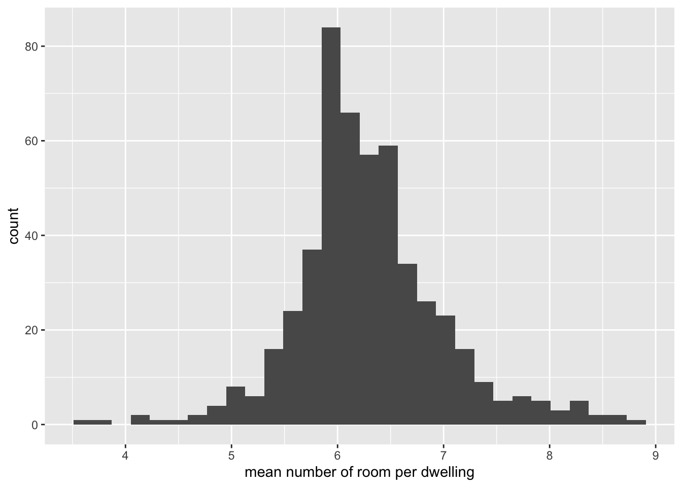

Code

Boston %>% 
    mutate(rm = as.integer(rm)) %>% 
    ggplot(aes(x=dis, y=medv, color=as.factor(rm))) +
    geom_smooth(method = 'lm', se = F) +
    labs(x = 'mean of distances to five Boston employment centers', y= 'median value of owner-occupied homes', color="mean number of room per dwelling") +
    theme(legend.position = 'bottom')

`geom_smooth()` using formula 'y ~ x'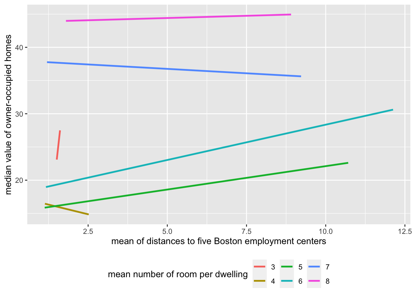

Thus, we added interaction term between dis and rm. The thumb of rule to use interaction term is hierarchical principle, which means, if we include an interaction in a model, we should also include the main effects, even if the p-values associated with main effect coefficients are not significant. Thus we should always use * instead of : when adding the interaction term. dis*rm means dis + rm + dis:rm.

Code

lm_wf3 <- workflow() %>% 
    add_model(lm_spec2) %>% 
    add_formula(medv ~ dis*rm + crim + chas)

lm_fit3 <- lm_wf3 %>% 
    fit(data = Boston)


lm_fit3 %>% 
    tidy()

# A tibble: 6 × 5
  term        estimate std.error statistic  p.value
  <chr>          <dbl>     <dbl>     <dbl>    <dbl>
1 (Intercept)   -5.03     4.70       -1.07 2.85e- 1
2 dis           -7.43     1.27       -5.84 9.30e- 9
3 rm             4.38     0.744       5.89 7.11e- 9
4 crim          -0.270    0.0341     -7.90 1.80e-14
5 chas           3.99     1.06        3.77 1.83e- 4
6 `dis:rm`       1.20     0.198       6.04 3.08e- 9

In this example, all predictors including interaction terms are significant. Interestingly, by adding the interaction between dis and rm, the coefficients associated with dis turn negative from positive when using simple single variable model. To interpret the interaction term,

dis:rm: since interaction term is significant (p-value = 3.077938e-09), thus linear relationship between dis and medv was significantly dependent on the rm, justifying the inclusion of the interaction term in the model.
dis: when there are 3 ~ 6 rooms in dwelling, one unit further away from five Boston employment centers, it results in $3,835 to $244 ((-7.426 + range(3,6) * 1.197) * 1000) decrease in median value of house. when there are more than 6 (7.426/1.197) rooms in dwelling, one unit further away from five Boston employment centers, it results in at least $953 ((-7.426 + 7 * 1.197) * 1000) increase in median value of house.
rm: keeping the mean distance to five Boston employment centers as constant dis, one more room in dwelling will increase 1000 * (1.197 * dis + 4.380) in the median value of house. Because the interaction term is positive (1.197), the rate of medv increase in terms of the room number will increase when it is further away from Boston employment centers.

When to use interaction term

The frequently asked question about interaction term is “when should we include interaction term”. The conventional answer is when two predictors are not independent. However, in reality, unless we have very strong prior knowledge about the predictors, it is hard to determine whether two predictors are dependent or not without exploring the data. From the articles/blogs about interaction term I read so far, two methods are generally used to determine whether add interaction term

try both with and without adding interaction term, if adding interaction term results in significance on interaction term, then use interaction term.
like what I did above, plot Y against X1 with X2 as nominal variable (if X2 is not nominal variable itself). If the lines from different X2 levels are parallel, then X1 and X2 are independent and no interaction terms are needed. Otherwise, add interaction term.

Logistic regression

In the regular linear regression mentioned above, the Y is numeric (aka. quantitative). However, when Y is nominal (aka, qualitative), logistic regression will be used. To make Y still represented by linear combination of predictors, we used logit function (link function) to transform Y (the probability) to $ln(\frac{p}{1-p})$ (the log odds).

\[ln(\frac{p}{1-p}) = \sum\beta X\] $\beta$ represents log odds ratio. thus, odds ratio $OR = e^\beta$.

When Y is binomial

To evaluate whether a customer will default the credit card default, we build a logistic model with three predictors – whether the customer is a student, the balance on the account and the customer income.

Again, for practice purpose, I used tidymodels syntax for demonstration.

Code

data("Default")
lr_spec <- logistic_reg() %>% 
    set_engine('glm') %>% 
    set_mode('classification')

default_wf <- workflow() %>% 
    add_model(lr_spec) %>% 
    add_formula(default ~ .)

default_fit <- default_wf %>% 
    fit(data = Default)

default_fit %>% 
    tidy()

# A tibble: 4 × 5
  term            estimate  std.error statistic   p.value
  <chr>              <dbl>      <dbl>     <dbl>     <dbl>
1 (Intercept) -10.9        0.492        -22.1   4.91e-108
2 studentYes   -0.647      0.236         -2.74  6.19e-  3
3 balance       0.00574    0.000232      24.7   4.22e-135
4 income        0.00000303 0.00000820     0.370 7.12e-  1

In this model, two predictors (student and balance) are significantly associated with default. To interpret coefficients, we first need to know which is the baseline of default.

Code

contrasts(Default$default)

    Yes
No    0
Yes   1

Based on the contrasts output, the baseline of default is No. Thus,

student: When keeping all other variable constant, compared to non-student (student = 0), a student (student = 1) is less likely to default credit card. The odds ratio is 0.524 (exp(-6.467758e-01)). In other words, if the odds of defaulting credit card as non-student is 1, the odds of defaulting credit card as a student is 0.524 (exp(-6.467758e-01)).
balance: When keeping all other variable constant, 1 dollar increase in account balance will result in increasing odds of 1.005 (exp(5.736505e-03)) to default credit card.

Note: above modeling is a bad model since there are high correlation between the predictors (collinearity). I just used it as an example to interpret the coefficients.

Multinominal predictors

Using multi-nominal predictor diagnosis and other predictors like sex and age time to predict whether the patient survived the brain cancer or not status

Code

data('BrainCancer')
BrainCancer <- BrainCancer %>% 
    na.omit()
contrasts(BrainCancer$diagnosis)

           LG glioma HG glioma Other
Meningioma         0         0     0
LG glioma          1         0     0
HG glioma          0         1     0
Other              0         0     1

In this example, Meningioma is the baseline for multi-nominal predictor diagnosis.

Code

BrainCancer_rec <- recipe(status ~ ., data = BrainCancer) %>% 
    step_mutate(status = as.factor(status)) %>% 
    step_dummy(diagnosis)
    
BrainCancer_wf <- workflow() %>% 
    add_model(lr_spec) %>% 
    add_recipe(BrainCancer_rec)

BrainCancer_fit <- BrainCancer_wf %>% 
    fit(data = BrainCancer)

BrainCancer_fit %>% 
    tidy()

# A tibble: 10 × 5
   term                estimate std.error statistic p.value
   <chr>                  <dbl>     <dbl>     <dbl>   <dbl>
 1 (Intercept)           3.56      2.57       1.39  0.166  
 2 sexMale               0.369     0.576      0.640 0.522  
 3 locSupratentorial     1.09      0.901      1.21  0.227  
 4 ki                   -0.0695    0.0326    -2.13  0.0332 
 5 gtv                   0.0382    0.0366     1.04  0.296  
 6 stereoSRT             0.253     0.771      0.328 0.743  
 7 time                 -0.0339    0.0155    -2.18  0.0291 
 8 diagnosis_LG.glioma   1.31      0.844      1.55  0.122  
 9 diagnosis_HG.glioma   2.37      0.778      3.05  0.00231
10 diagnosis_Other       0.765     0.940      0.814 0.416

For multi-nominal predictor diagnosis, the levels (LG glioma, HG glioma and Other) are compared to the baseline Meningioma, and it ends with three terms for coefficient estimation.

Based on above model, only HG glioma show significant association with survival (p-value < 0.05) when choose Meningioma as baseline. When keeping all other variable constant, compare to Meningioma, the patient with HG glioma are 10 times more (exp(2.37027243)) likely to survive. If we want to compare HG glioma with Other cancer type, simply use exp(2.37027243-0.76482440) to get odds ratio between HG glioma and Other, in which compare to Other, the patient with HG glioma are 5 times more (exp(2.37027243-0.76482440)) likely to survive. However, in this case, we do not know whether this comparison is statistically significant. We can get p-value for this comparison by switching Other as baseline.

Contrasts matrix

Another baseline assignment is using the global average as baseline. To do that, we need to change the contrasts matrix. The following code replace the default contrasts contr.treatment with contr.sum on globalOptions, then use step_dummy from recipe to realize it

Code

BrainCancer_rec %>% 
    prep() %>% 
    bake(new_data = NULL, starts_with("diagnosis")) %>% 
    mutate(diagnosis_orginal = BrainCancer$diagnosis) %>% 
    distinct()

# A tibble: 4 × 4
  diagnosis_LG.glioma diagnosis_HG.glioma diagnosis_Other diagnosis_orginal
                <dbl>               <dbl>           <dbl> <fct>            
1                   0                   0               0 Meningioma       
2                   0                   1               0 HG glioma        
3                   1                   0               0 LG glioma        
4                   0                   0               1 Other

Code

contr_opt <- getOption("contrasts")
contr_opt

        unordered           ordered 
"contr.treatment"      "contr.poly"

The original baseline is Meningioma, each diagnosis_ is compared to the Meningioma.

Code

contr_sum_opt <- contr_opt
contr_sum_opt['unordered'] <- 'contr.sum'
options(contrasts = contr_sum_opt)

# my_naming <- function(var, lvl, ordinal = FALSE, sep = "_"){
#     paste(var, levels(BrainCancer$diagnosis)[lvl])
# }

BrainCancer_rec2 <- recipe(status ~ ., data = BrainCancer) %>% 
    step_mutate(status = as.factor(status)) %>% 
    step_dummy(diagnosis)
    
BrainCancer_rec2 %>% 
    prep() %>% 
    bake(new_data = NULL, starts_with("diagnosis")) %>% 
    mutate(diagnosis_orginal = BrainCancer$diagnosis) %>% 
    distinct()

# A tibble: 4 × 4
  diagnosis_X1 diagnosis_X2 diagnosis_X3 diagnosis_orginal
         <dbl>        <dbl>        <dbl> <fct>            
1            1            0            0 Meningioma       
2            0            0            1 HG glioma        
3            0            1            0 LG glioma        
4           -1           -1           -1 Other

Thus diagnosis_X1, diagnosis_X2 and diagnosis_X3 now represents Meningioma, HG glioma and LG glioma compared to average baseline.

Code

BrainCancer_wf2 <- workflow() %>% 
    add_recipe(BrainCancer_rec2) %>% 
    add_model(lr_spec)

BrainCancer_fit2 <- BrainCancer_wf2 %>% 
    fit(data = BrainCancer)

BrainCancer_fit2 %>% 
    tidy()

# A tibble: 10 × 5
   term         estimate std.error statistic p.value
   <chr>           <dbl>     <dbl>     <dbl>   <dbl>
 1 (Intercept)    5.52      2.66       2.07   0.0380
 2 sex1          -0.184     0.288     -0.640  0.522 
 3 loc1          -0.545     0.451     -1.21   0.227 
 4 ki            -0.0695    0.0326    -2.13   0.0332
 5 gtv            0.0382    0.0366     1.04   0.296 
 6 stereo1       -0.127     0.386     -0.328  0.743 
 7 time          -0.0339    0.0155    -2.18   0.0291
 8 diagnosis_X1  -1.11      0.468     -2.37   0.0177
 9 diagnosis_X2   0.195     0.594      0.329  0.742 
10 diagnosis_X3   1.26      0.542      2.33   0.0200

Based on the newly trained model BrainCancer_fit2, only Meningioma and LG glioma show significant association with survival (p-value < 0.05) when compared to global average. When keeping all other variable constant, compare to global average, the patient with Meningioma has only 32.9% (exp(-1.11018843)) average survive rate, while the patient with LG glioma are 3.5 times (exp(1.26008400)) more likely to survive.

More about coding contrasts in base R syntax can be found at this article.

Multinomial outcome

Using the same dataset BrainCancer, now I try to predict the diagnosis based on the tumor location (loc), Karnofsky index (ki), Gross tumor volume (gtv) and Stereotactic method (stereo). Here we used multinom_reg() to model multinomial regression

Code

options(contrasts = contr_opt) # reset contrasts options back to `contr.treatment`

ml_spec <- multinom_reg() %>% 
    set_engine('nnet') %>% 
    set_mode('classification')

BrainCancer_rec3 <- recipe(diagnosis ~ loc + ki + gtv + stereo, data = BrainCancer) %>% 
    update_role(diagnosis, new_role = 'outcome') %>% 
    step_normalize(all_numeric_predictors()) %>% 
    step_dummy(all_nominal_predictors())

BrainCancer_wf3 <- workflow() %>% 
    add_model(ml_spec) %>% 
    add_recipe(BrainCancer_rec3)

BrainCancer_fit3 <- BrainCancer_wf3 %>% 
    fit(data = BrainCancer)

BrainCancer_fit3

══ Workflow [trained] ══════════════════════════════════════════════════════════
Preprocessor: Recipe
Model: multinom_reg()

── Preprocessor ────────────────────────────────────────────────────────────────
2 Recipe Steps

• step_normalize()
• step_dummy()

── Model ───────────────────────────────────────────────────────────────────────
Call:
nnet::multinom(formula = ..y ~ ., data = data, trace = FALSE)

Coefficients:
          (Intercept)          ki         gtv loc_Supratentorial stereo_SRT
LG glioma  -2.3035689  0.23860763 -0.02596393          0.3998414  0.5444269
HG glioma  -2.5894735  0.03684929  0.15897113          0.9417737  1.3658683
Other      -0.4158848 -0.29780559  0.14203552         -2.7892771  1.4289732

Residual Deviance: 187.5196 
AIC: 217.5196

In the multinomial regression, no p-value were reported. The coefficients represent log odds ratio.

Each row in the coefficient table corresponds to the model equation. eg. the first row represents the coefficients for LG glioma in comparison to our baseline Meningioma. Each column in the coefficient table corresponds to specific coefficient estimate. Thus, compared to Meningioma, using SRT Stereotactic method is about 4 times (exp(1.3658683)) more likely diagnose HG glioma. A tumor is only 6% (exp(-2.7892771)) chance to be diagnosed as Other instead of Meningioma if it is located at Supratentorial area.

To perform above model in base R syntax, please refer to the blog post by Mohit Sharma.

Poisson regression

Poisson regression is used to model count outcome. Unlike regular linear regression, count outcome is not real continuous variable. Instead, it must be positive integer and usually modeled by Poisson distribution rather than normal distribution.

The link function for Poisson regression is log function $\ln\lambda$ where $\lambda$ represents the mean of outcome.

In the following example, we use Bikeshare data to predict bikers outcome which represents the count of rental bikers

Code

data('Bikeshare')

Bikeshare_rec <- recipe(bikers ~ season + weekday + weathersit + temp + hum + windspeed, data = Bikeshare) %>% 
    step_num2factor(season, levels = c("winter",'spring','summer','fall')) %>%
    step_num2factor(weekday, transform = function(x) {x+1}, levels = c('sunday','monday','tuesday','wednesday','thursday','friday','saturday')) %>%
    step_normalize(all_numeric_predictors()) %>%
    step_dummy(all_nominal_predictors()) %>%
    I()

# Bikeshare_rec %>% prep() %>% bake(new_data = NULL)
library(poissonreg)
pr_spec <- poisson_reg() %>% 
    set_engine('glm') %>% 
    set_mode('regression')

Bikeshare_wf <- workflow() %>% 
    add_recipe(Bikeshare_rec) %>% 
    add_model(pr_spec)

Bikeshare_fit <- Bikeshare_wf %>%
     parsnip::fit(Bikeshare)

Bikeshare_fit %>%
    tidy()

# A tibble: 16 × 5
   term                       estimate std.error statistic   p.value
   <chr>                         <dbl>     <dbl>     <dbl>     <dbl>
 1 (Intercept)                  4.58    0.00385   1191.    0        
 2 temp                         0.426   0.00149    285.    0        
 3 hum                         -0.256   0.00108   -238.    0        
 4 windspeed                    0.0404  0.000949    42.6   0        
 5 season_spring                0.302   0.00384     78.7   0        
 6 season_summer                0.144   0.00449     32.1   1.12e-226
 7 season_fall                  0.613   0.00345    177.    0        
 8 weekday_monday              -0.0464  0.00336    -13.8   1.82e- 43
 9 weekday_tuesday             -0.0405  0.00336    -12.1   1.42e- 33
10 weekday_wednesday           -0.0524  0.00342    -15.3   4.88e- 53
11 weekday_thursday            -0.0804  0.00339    -23.7   2.70e-124
12 weekday_friday              -0.0151  0.00335     -4.51  6.47e-  6
13 weekday_saturday            -0.0187  0.00336     -5.58  2.36e-  8
14 weathersit_cloudy.misty      0.106   0.00223     47.4   0        
15 weathersit_light.rain.snow  -0.163   0.00425    -38.4   0        
16 weathersit_heavy.rain.snow  -0.0368  0.167       -0.221 8.25e-  1

Code

contrasts(Bikeshare$weathersit)

                cloudy/misty light rain/snow heavy rain/snow
clear                      0               0               0
cloudy/misty               1               0               0
light rain/snow            0               1               0
heavy rain/snow            0               0               1

All terms except weathersit_heavy.rain.snow are significantly associated with rental bikers number. - when keeping all other variables constant, compared to season_winter, season_spring will increase the mean of rental biker count by 1.35 exp(0.30234965). In other words, there will be 135% bikers rental a bike in spring than winter. - when keeping all other variables constant, every unit increase in temperature will result in on average 1.53 (exp(0.42588059)) rental biker customer.

note:above model is not optimal model to predict rental bikers. We use the model without interactions to simplify the question and emphasize interpretation of coefficients in the context of poisson regression . To interpret the coefficients with interaction term, refer to previous regular linear regression example

Final remarks

In this post, I focus on interpret the coefficients in three GLM, and show the examples of coefficients associated with both quantitative and qualitative predictors. I also include the examples to interpret coefficients when 1) add interaction term, 2) with multi-nominal outcome and 3) with alternative contrast matrix.