Network Analysis in R - Part 2

network

Author

Chun Su

Published

August 24, 2019

In last post, I covered the basic components of IGRAPH objects and how to manipulate IGRAPH. You may notice that most of those manipulation do not really require a IGRAPH object to play with. However, in this post, you will realize the advantage of using IGRAPH over data.frame in network analysis.

In this session, we are going to use a new un-directed graph called gr generated by sample_gnp().

Code

library(igraph)
library(tidyverse)
library(ggraph)
library(gridExtra)

Code

# generate random graph 
set.seed(12) 
gr <- sample_gnp(10, 0.3)
plot(gr)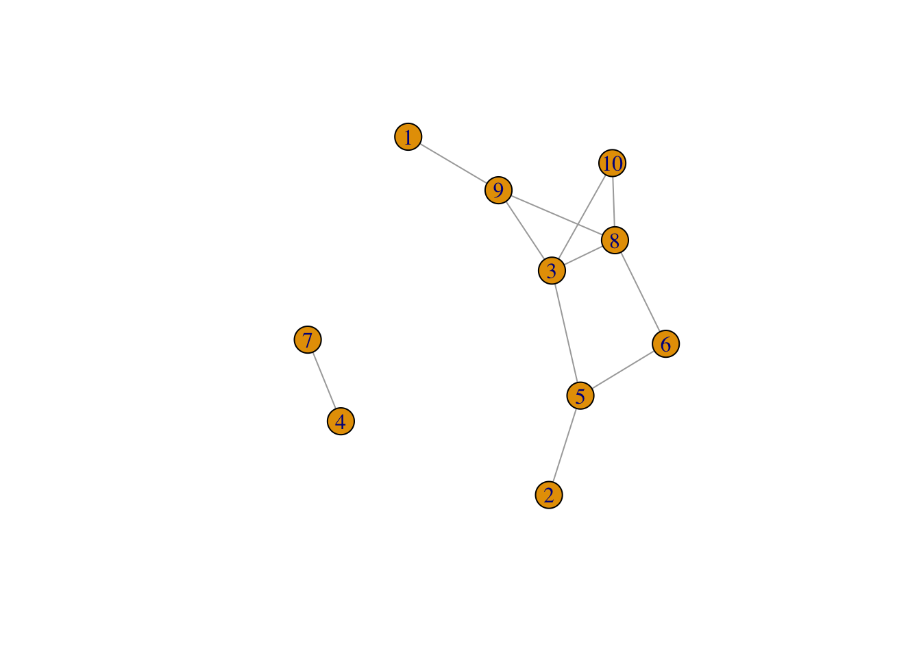

Graph measurement

Degree and strength

Degree measures the number of edges connected to given vertex. In igraph, we use degree. Be aware that, for directed graph, the node degree can be “in-degree” (the edge number pointing to the node) and “out-degree” (the edge number pointing from node). We can also summaries the all degree by using degree_distribution.

Code

# get degree for each node 
degree(gr, v=1:10)

 [1] 1 1 4 1 3 2 1 4 3 2

Code

# degree distribution
degree_distribution(gr) # probability for degree 0,1,2,3,4

[1] 0.0 0.4 0.2 0.2 0.2

strength is weighted version of degree, by summing up the edge weights of the adjacent edges for each vertex.

Code

# add random weight attribute
set.seed(12)
gr2 <- gr %>% set_edge_attr(
  "weight",index=E(gr),
  value=sample(seq(0,1,0.05),size=length(E(gr)))
)
# calculate strength
strength(gr2, weights = E(gr)$weight)

 [1] 1.00 0.05 2.65 0.20 1.45 1.20 0.20 2.85 1.85 1.65

Order/distance and path

Order measures the edge number from one node to the other. In igraph package, we use distances function to get order between two vertices. For directed graph, in mode only follow the paths toward the first node, while out mode goes away from the first node. If no connection can be made, Inf will be return.

Code

# count all edges from 1 to 10, regardless of direction 
distances(gr, v=1, to=10, mode="all", weights = NA)

     [,1]
[1,]    3

Code

# pairwise distance table 
distances(gr, mode="all")

      [,1] [,2] [,3] [,4] [,5] [,6] [,7] [,8] [,9] [,10]
 [1,]    0    4    2  Inf    3    3  Inf    2    1     3
 [2,]    4    0    2  Inf    1    2  Inf    3    3     3
 [3,]    2    2    0  Inf    1    2  Inf    1    1     1
 [4,]  Inf  Inf  Inf    0  Inf  Inf    1  Inf  Inf   Inf
 [5,]    3    1    1  Inf    0    1  Inf    2    2     2
 [6,]    3    2    2  Inf    1    0  Inf    1    2     2
 [7,]  Inf  Inf  Inf    1  Inf  Inf    0  Inf  Inf   Inf
 [8,]    2    3    1  Inf    2    1  Inf    0    1     1
 [9,]    1    3    1  Inf    2    2  Inf    1    0     2
[10,]    3    3    1  Inf    2    2  Inf    1    2     0

To get detail route from one node to the other, we use path.

Code

# shortest path to connect
all_shortest_paths(gr, 1,10)$res

[[1]]
+ 4/10 vertices, from bd1187d:
[1]  1  9  8 10

[[2]]
+ 4/10 vertices, from bd1187d:
[1]  1  9  3 10

Code

# all path to connect
all_simple_paths(gr, 1,10)

[[1]]
+ 7/10 vertices, from bd1187d:
[1]  1  9  3  5  6  8 10

[[2]]
+ 5/10 vertices, from bd1187d:
[1]  1  9  3  8 10

[[3]]
+ 4/10 vertices, from bd1187d:
[1]  1  9  3 10

[[4]]
+ 5/10 vertices, from bd1187d:
[1]  1  9  8  3 10

[[5]]
+ 7/10 vertices, from bd1187d:
[1]  1  9  8  6  5  3 10

[[6]]
+ 4/10 vertices, from bd1187d:
[1]  1  9  8 10

Transitivity

Transitivity measures the probability that the adjacent vertices of a vertex are connected. This is also called the clustering coefficient, a proxy to determine how well connected the graph is. This property is very important in social networks, and to a lesser degree in other networks.

Code

# two extreme classes -- full graph and ring graph
g1 = make_full_graph(10)
plot(g1)

Code

transitivity(g1)

[1] 1

Code

g2 = make_ring(10)
plot(g2)

Code

transitivity(g2)

[1] 0

There are multiple different types of transitivity can be calculated (weighted or un-weighted). Also, the transitivity can be calculated locally for a sub-graph by specifying vertex ids. See details by ?transitivity

Centrality

Centrality indices identify the most important vertices within a graph. In other words, the “hub” of network. However, this “importance” can be conceived in two ways:

relation to a type of flow or transfer across the network.
involvement in the cohesiveness of the network

The simplest of centrality indicator is degree centrality (centr_degree), aka, a node is important if it has most neighbors.

Besides degree centrality, there are

closeness centrality (centr_clo) - a node is important if it takes the shortest mean distance from a vertex to other vertices
between-ness centrality (centr_betw) - a node is important if extent to which a vertex lies on paths between other vertices are high.
eigenvector centrality (centr_eigen) - a node is important if it is linked to by other important nodes.

Code

centr_degree(gr, mode="all")

$res
 [1] 1 1 4 1 3 2 1 4 3 2

$centralization
[1] 0.2

$theoretical_max
[1] 90

Code

centr_clo(gr, mode = "all")

$res
 [1] 0.3888889 0.3888889 0.7000000 1.0000000 0.5833333 0.5384615 1.0000000
 [8] 0.6363636 0.5833333 0.5000000

$centralization
[1] 0.8690613

$theoretical_max
[1] 4.235294

Code

centr_betw(gr, directed = FALSE)

$res
 [1] 0.0 0.0 8.0 0.0 6.5 1.0 0.0 4.5 6.0 0.0

$centralization
[1] 0.1666667

$theoretical_max
[1] 324

Code

centr_eigen(gr,directed = FALSE)

$vector
 [1] 2.519712e-01 1.933127e-01 1.000000e+00 2.093280e-17 5.762451e-01
 [6] 5.244145e-01 1.036823e-17 9.869802e-01 7.511000e-01 6.665713e-01

$value
[1] 2.980897

$options
$options$bmat
[1] "I"

$options$n
[1] 10

$options$which
[1] "LA"

$options$nev
[1] 1

$options$tol
[1] 0

$options$ncv
[1] 0

$options$ldv
[1] 0

$options$ishift
[1] 1

$options$maxiter
[1] 1000

$options$nb
[1] 1

$options$mode
[1] 1

$options$start
[1] 1

$options$sigma
[1] 0

$options$sigmai
[1] 0

$options$info
[1] 0

$options$iter
[1] 8

$options$nconv
[1] 1

$options$numop
[1] 26

$options$numopb
[1] 0

$options$numreo
[1] 16


$centralization
[1] 0.6311756

$theoretical_max
[1] 8

Many other centrality indicators refer to wiki page of Centrality.

Graph clustering

Graph clustering is the most useful calculation that can be done in igraph object. There are a whole line of research on this. Only basic clustering methods were covered here.

decompose graph

To split graph into connected sub-graph, decompose.graph calculates the connected components of your graph. A component is a sub-graph in which all nodes are inter-connected.

Code

# decompose graph to connected components
dg <- decompose.graph(gr)
dg

[[1]]
IGRAPH a672a32 U--- 8 10 -- Erdos-Renyi (gnp) graph
+ attr: name (g/c), type (g/c), loops (g/l), p (g/n)
+ edges from a672a32:
 [1] 2--4 3--4 4--5 3--6 5--6 1--7 3--7 6--7 3--8 6--8

[[2]]
IGRAPH f52a970 U--- 2 1 -- Erdos-Renyi (gnp) graph
+ attr: name (g/c), type (g/c), loops (g/l), p (g/n)
+ edge from f52a970:
[1] 1--2

Code

# summary statics graph components
components(gr)

$membership
 [1] 1 1 1 2 1 1 2 1 1 1

$csize
[1] 8 2

$no
[1] 2

Code

# plot components
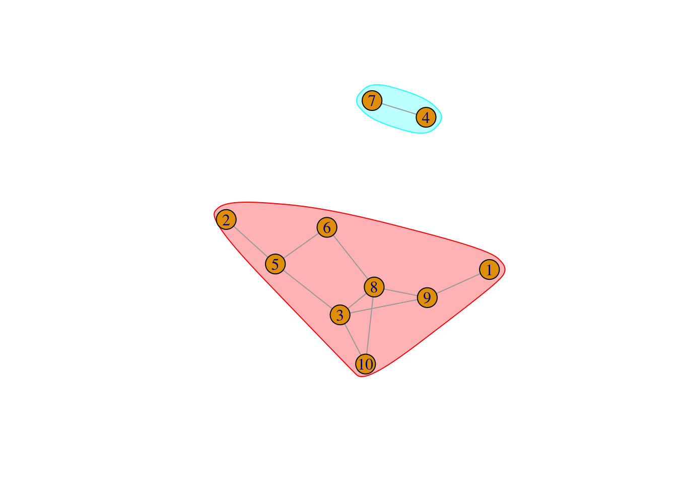
coords <- layout_(gr, nicely())
plot(gr, layout=coords,
     mark.groups = split(as_ids(V(gr)), components(gr)$membership)
     )

Cliques

Clique is a special sub-graph in which every two distinct vertices are adjacent. The direction is usually ignored for clique calculations

Code

# extract cliques that contain more than 3 vertices
cliques(gr, min=3)

[[1]]
+ 3/10 vertices, from bd1187d:
[1]  3  8 10

[[2]]
+ 3/10 vertices, from bd1187d:
[1] 3 8 9

Code

# get cliques with largest number of vertices
largest_cliques(gr)

[[1]]
+ 3/10 vertices, from bd1187d:
[1] 8 3 9

[[2]]
+ 3/10 vertices, from bd1187d:
[1]  8  3 10

Code

# plot cliques
cl <- cliques(gr, 3)

coords <- layout_(gr, nicely())
plot(gr, layout=coords,
     mark.groups=lapply(cl, function(g){as_ids(g)}), 
     mark.col=c("#C5E5E7","#ECD89A"))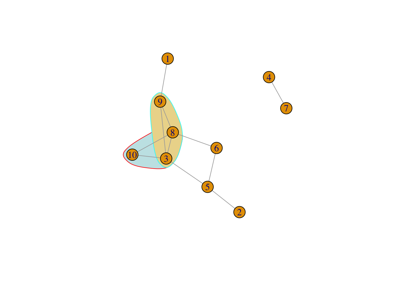

Communities and modules

Graph communities structure is defined if the nodes of the network can be easily grouped into (potentially overlapping) sets of nodes such that each set of nodes is densely connected internally. Modularity is always used as a measure the strength of division of a network into community for optimization methods in detecting community structure in networks.

There are many algorithms to cluster graph to communities.

cluster_edge_betweenness a hierarchical decomposition process where edges are removed in the decreasing order of their edge betweenness scores.
cluster_optimal - a top-down hierarchical approach that optimizes the modularity function
cluster_walktrap - an approach based on random walks
cluster_fast_greedy
cluster_label_prop
cluster_leading_eigen
cluster_Louvain
cluster_spinglass

Which cluster method to use? Refer to this stackoverflow post for more information.

Code

# cluster graph using walktrap method, turn a ”communities” object
wtc <- cluster_walktrap(gr) 
wtc

IGRAPH clustering walktrap, groups: 3, mod: 0.33
+ groups:
  $`1`
  [1]  1  3  8  9 10
  
  $`2`
  [1] 2 5 6
  
  $`3`
  [1] 4 7

Code

# find membership for each vertex
membership(wtc)

 [1] 1 2 1 3 2 2 3 1 1 1

Code

# calculate modularity for walktrap clustering on this graph
modularity(wtc)

[1] 0.3305785

Code

# plot community
coords <- layout_(gr, nicely())
plot(wtc, gr, layout=coords)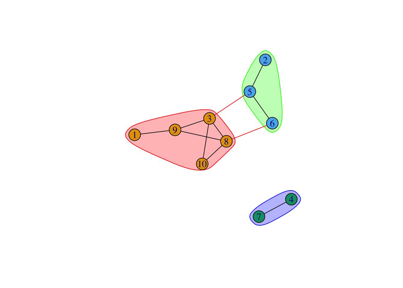

To learn more about graph clustering: